ZFit: How to have confidence in results using std err.?

Introduction

Fitting data obtained with Electrochemical Impedance Spectroscopy (EIS) measurements leads to the determination of the parameters values of an equivalent circuit model whose impedance can be considered equivalent to that of the electrochemical system under study.
Agreement between experimental data and simulated data from the fitting procedure, is called “goodness of fit” or “quality of fit”. This agreement is evaluated by the $\chi^2$ parameter: the lower, the better.

This parameter ($\chi^2$) is calculated using the sum of the residuals, i.e. the difference between the experimental impedance values and the simulated impedance values resulting from the fit. The minimization algorithm finds the set of parameters’ values for which $\chi^2$ is minimal.

How much confidence can you have in these values? How do you know if the parameter is relevant or not?
Partial answers to these questions are given by the “std err.” parameter, which you can find next to the unit of the parameter in the Results section of the ZFit main window (Fig. 1).

Figure 1: The std err. parameter in the Results section of the ZFit window.

What is it?

In EC-Lab, “std err.” stands for standard error. The standard error measures the extent of uncertainty related to the parameter’s value estimated by the minimization algorithm. This error is mainly due to:

• Measurement errors (random and systematic).
• An inadequate equivalent circuit.
• An unsuccessful minimization procedure.

 
The standard error can be represented in terms of a Probability Density Function (PDF) (Fig. 2), and it is symbolized by $\sigma$. The mean value $\mu$ represents the estimated value of the parameter considered (equal to 0 for the sake of simplicity [1]).

The percentages shown in Figure 1 quantify the probability that the parameter’s true value lies within the defined area, assuming it follows Gaussian or Normal law. The probability that the measured value falls within an interval of [$\mu-2\sigma$; $\mu+2\sigma$], is approximately 95%, for a coverage factor $k=2$.*“The coverage factor is a number larger than one by which a combined standard measurement uncertainty is multiplied to obtain an expanded measurement uncertainty” JCGM 200:2008 International vocabulary of metrology — Basic and general concepts and associated terms (VIM). Because the true value can never be reached, we can only reason in terms of probability and value intervals. The probability that the true value falls between [-$\infty$;+$\infty$] is of course 100%.

Figure 2: Probability Density Function (PDF) of a parameter whose value follows a Gaussian or Normal statistical distribution with a mean equal to 0 and a standard error equal to σ. The probability that the true value of this parameter is between -σ and σ is 68.2%.

Using the standard error, the confidence interval*According to “JCGM 200:2008 International vocabulary of metrology — Basic and general concepts and associated terms (VIM)”, it should be preferable to use the term “coverage interval”, which is defined as “the interval containing the set of true quantity values of a measure and with a stated probability, based on the information available.”can be calculated, considering it is given for a probability of 95.6 %. It is shown in Figure 3 for the parameter R3 using the std error calculated by fitting the data (Fig. 1). The confidence interval is [R3 – 2 std. err.; R3 + 2 std. err.], i.e. ca. [0.0350; 0.0360] with R3 = 0.03547.

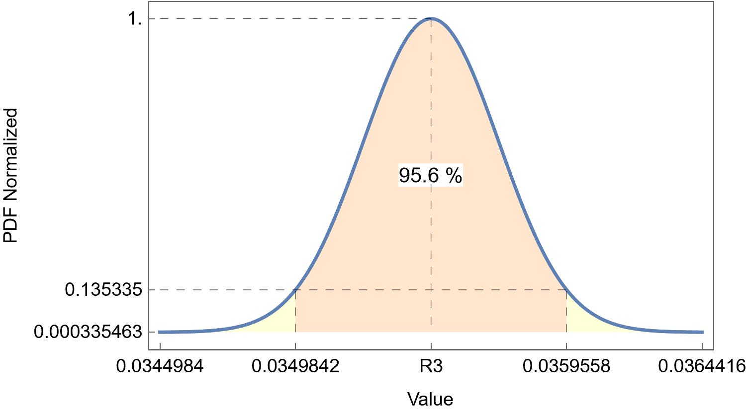
Figure 3: Normalized Probability Density Function (PDF) of a Gaussian distribution with the value of the parameter R3 in Fig. 1 as a mean $\mu$ and std err. as a standard deviation. The confidence interval is shown in light orange.

How is it calculated?

There are several ways to calculate the standard error for non-linear regression problems: covariance matrix, bootstrap, jackknife, Monte-Carlo…

Since EC-Lab^® 11.50, we are using an adapted Monte-Carlo method following the paper by Joseph S. Alper and Robert I. Gelb [2], which is described below.

The fitting procedure is performed on one set of data (one “trial”), but as we have seen above, the standard deviation or error is a statistical parameter, which requires many data sets (many “trials”). ZFit effectively creates a population of data sets.

After the initial minimization procedure using the method and criteria shown in Fig. 4, Box 1, the residuals are used to simulate other data that are then fitted again using the stop criteria that have been defined. The minimization results in new parameters values. The number of new simulated data (and new parameters values) is indicated by the number in the simulation box (Fig. 4, Box 2). From this set of parameters values, the standard error is calculated.

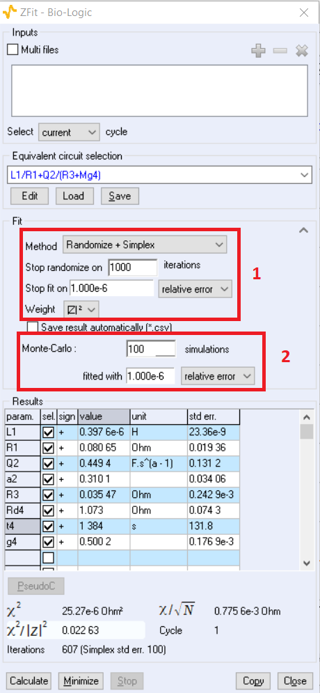
Figure 4: ZFit window showing the parameters for the std err. calculation. The number of simulations corresponds to the number of parameter values used to calculate the standard error.

Examples

Effect of measurement noise on the standard error

Using Mathematica computing software [3], we simulated 7 impedance data sets at the same frequencies and increasing noise amplitude. We imported the data into EC-Lab^® using the “Import file” function. Figure 5 shows the various graphs, where the chosen “theoretical” equivalent circuit was R1 + R2/C2 with R1 = 1000 Ω, R2 = 500 Ω, C2 = 1 µF.

To simulate noisy data, a value randomly picked in a Gaussian distribution with an increasing standard deviation and a mean of zero, was added at each frequency to the real part and the imaginary part of the impedance.

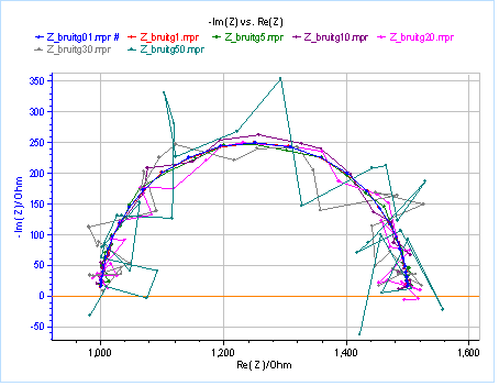
Figure 5: Simulated impedance graphs with random noise of increasing amplitudes.

The effect of the additional noise can be seen in the value of std err. that results from fitting the data with R1+C2/R2 equivalent circuit. This is illustrated in Fig. 6, where the confidence interval at 95% is represented as an error bar of std err. around the calculated parameter value. As the noise increases, the std err. increases and the confidence interval broadens for the three different parameters (R1, R2, and C1). It can be seen that additional noise not only affects the precision of the measurement, illustrated by the confidence interval, but also the accuracy of the measurement, illustrated by the fact that the calculated parameter values move farther from the theoretical or true parameter value (red lines in Fig. 6). For a noise of standard deviation 20, the true value seems to be at the very edge of the confidence interval.

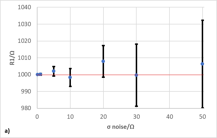
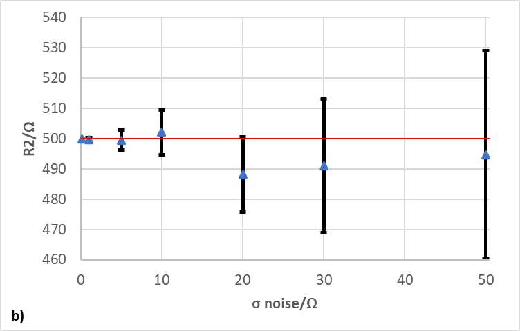
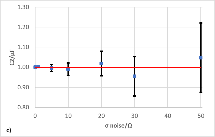
Figure 6: Evolution of the value of the parameter and the std err. with the noise amplitude for a) R1, b) R2, and c) C2. The error bars represent the standard errors given in ZFit. The red lines represent the theoretical, or in this case, true values of the parameter.

Complex equivalent circuit

The std err. can also be used to indicate that one or more components might not be relevant in the equivalent circuit used to fit the data. To prove this point, we used the data shown in reference [4, Fig. 3], that we simulate using ZSim and the equivalent circuit proposed in the paper [4, Fig. 2]. The data were fitted, and the results are given in Fig. 7. Figure 7 shows two different fitting procedures leading to two different aberrant parameters: in Fig. 7a, the parameters R5 and C5 seem to be aberrant because the standard errors are larger than their values. In Fig. 7b, the parameters C2 and R2 also seem to be aberrant for the same reason. It is not surprising that the same fitting procedure leads to different results because it is well-known that the circuit C1/R1+C2/R2 is equivalent to C1/(R1+C2/R2). To learn more about distinguishability of equivalent circuit, please visit the Learning Center article: ZSim and ZFit as learning tools. Part VI – Equivalent circuits distinguishability

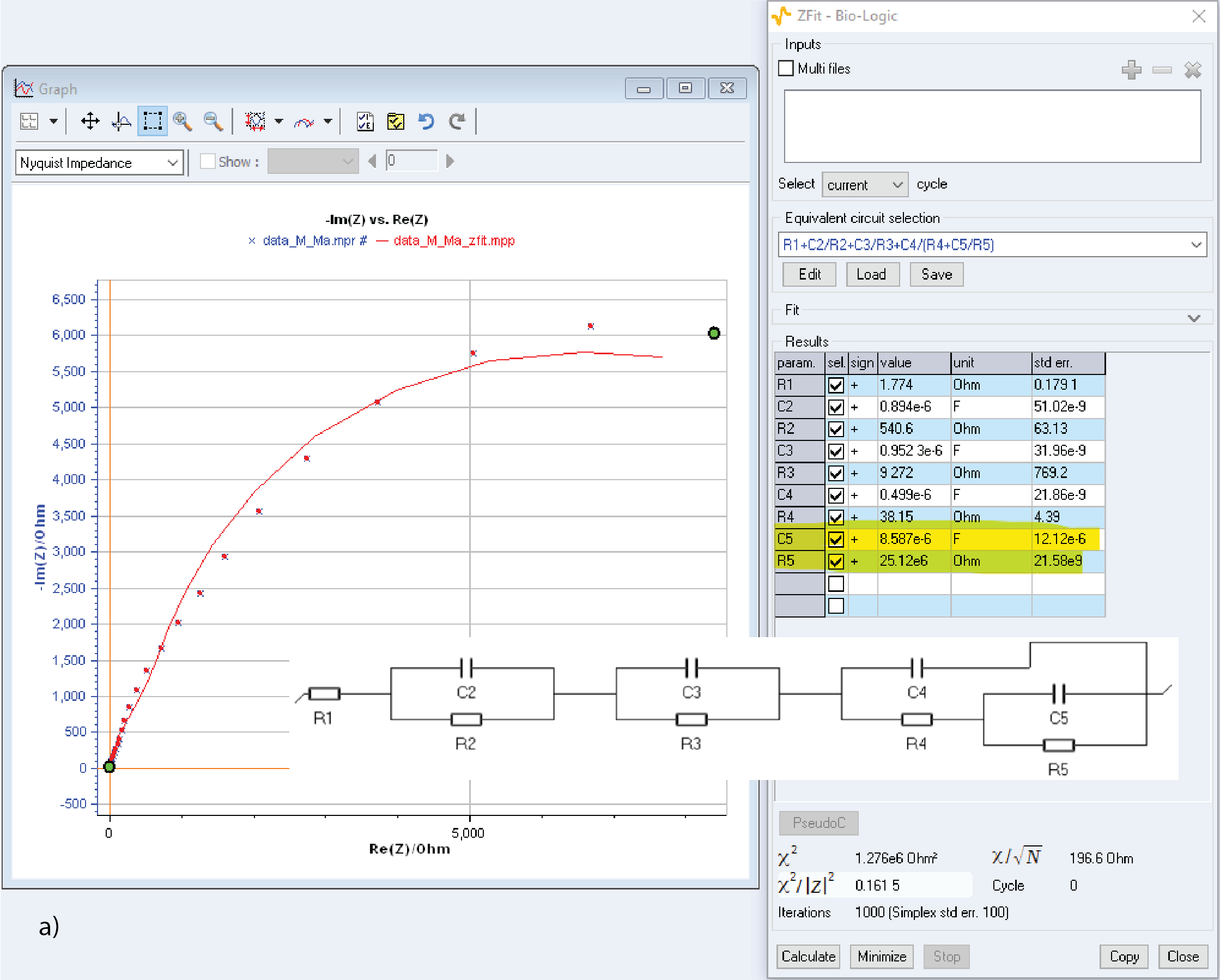
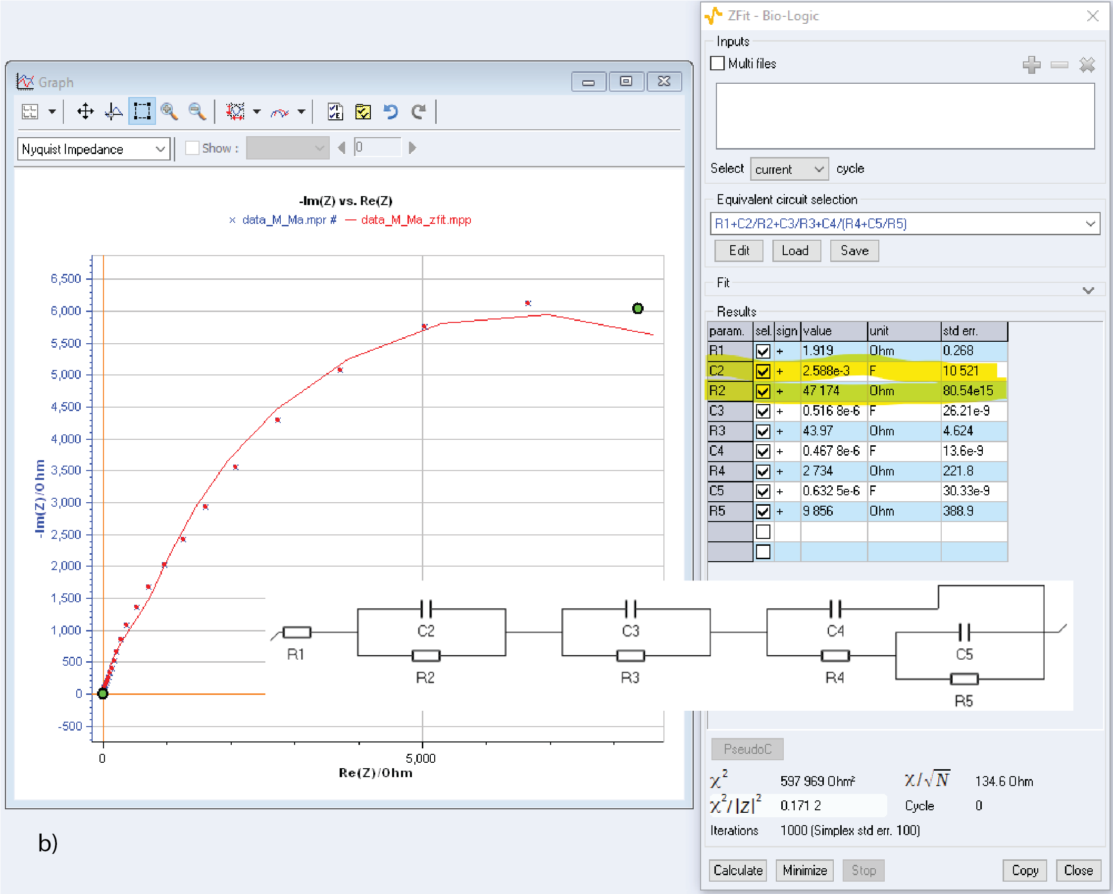
Figure 7: Simulated data from [4] fitted using the equivalent circuit proposed in the paper, a) and b) show two different fitting results with two different aberrant sets of parameters.

Figure 8 shows fitting results using an equivalent circuit obtained by removing a) R5 and C5 and b) C2 and R2. For both fitting results there are no aberrant parameters and the $\chi^2/|Z|^2$ parameter, which quantifies the goodness of the fit, is only slightly larger than in Fig. 7. In Figs. 8a and 8b all the parameters seem to be significant and relevant, all standard errors being smaller than the parameters values.
It must be added that the equivalent circuit shown in Fig. 8b should be preferred because it is identifiable, which means the value of the elements can be univocally determined whereas the circuit shown in Fig. 8a is not identifiable: from one fit to another, R2 and C2 could take the values of R3 and C3 for example, or of R4 and C4. More about a circuit’s identifiability can be found here: ZSimand ZFit as learning tools. Part VII – Equivalent circuits identifiability

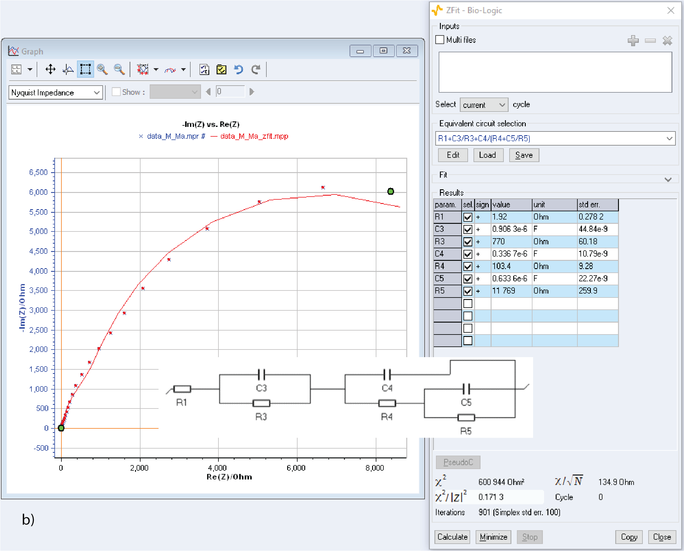
Figure 8: Simulated data from [3] fitted using modified and simplified equivalent circuits: a) Voigt-type equivalent circuit b) Ladder-type equivalent circuit.

Incomplete impedance data

Finally, we would also like to show how fitting incomplete impedance data affects the determination of the parameter value and its standard error.

Using ZSim, the impedance simulation software in EC-Lab^®, we simulated five impedance data sets corresponding to the impedance of the element M, which models the restricted diffusion process [5]. For each data set, the minimum frequency was increased, while the parameter values and the number of points remained constant. The evolution of the Nyquist diagram can be seen in Fig. 9, as the minimum frequency increases, the data become more truncated.

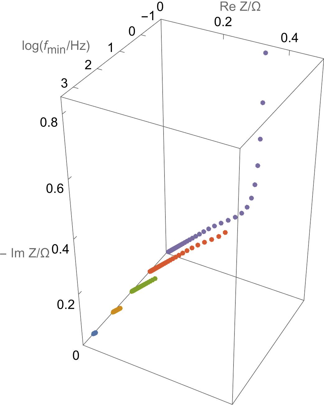
Figure 9: Nyquist diagrams of simulated impedance data obtained with ZSim. The impedance of the element M is simulated with the following parameters: Rd = 1 Ohm and td = 1 s. The minimum frequency decreases and the data become less and less truncated.

Each data set was fitted using ZFit and the element M. The evolution of the value of the parameters and their standard errors are shown in Figs. 10a and 10b, respectively.
In Fig. 10a, it can be seen that even though data are truncated by two decades $\left(f_\text{min} = 10\, \text{Hz}\right)$ both parameters Rd and td are correctly determined. The standard error (Fig. 10b) increases to three orders of magnitude when the minimum frequency is equal to 1 Hz, which shows that it is more “sensitive” to incomplete data than the parameter value. When even more data points are missing, the parameter values deviate farther from the true values and the standard error also largely increase. Interestingly, the standard error decreases when the found parameter values are close to 0. In this case, all data are concentrated into a very small value domain.

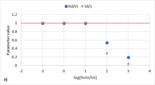
Figure 10: Evolution of a) the value of the parameter and b) the standard error vs. minimum frequency of the simulated M impedance data. The red line represents the true values of the parameters.

Published 05/2023

References

[1] https://en.wikipedia.org/wiki/Standard_deviation (Accessed on October 26th 2022)
[2] J. S. Alper and R. I. Gelb Standard Errors and Confidence Intervals in Nonlinear Regression: Comparison of Monte Carlo and Parametric Statistics J. Phys. Chem. (1990), 94, 4741-4151
[3] Wolfram Research, Inc., Mathematica, Version 13.2, Champaign, IL (2022).
[4] Ma, M., Yang, C.-X., Cai, W.-B., Zhou, W.-F., and Liu, H.-T. Oxidation kinetics of a lead electrode covered with an anodic Pb(II) film in sulfuric acid solution J. Electrochem. Soc. (2003), 150, 7 B325.
[5] Handbook of Electrochemical Impedance Spectroscopy. DIFFUSION IMPEDANCES – [PDF]