How to check and correct the time variance of your system under EIS measurements

Why is time-variance problematic for Electrochemical Impedance Spectroscopy (EIS) measurements?

Compare an EIS measurement with taking a picture. You can compare camera exposure time with frequency: high frequencies correspond to short exposure time and low frequencies to long exposure times. The whole point of a measurement (or a photograph), in most cases, is to capture a moment in time. If an object is moving, it will be easy to capture this moment if the exposure is short enough. If it is dark and you need more light, you will also need a longer exposure. If the object is moving, with a longer exposure, it will appear blurred.

Well, the time-variance of a system is the same as the movement of an object. At low frequencies, as the system is changing, you are not sure what is the actual system that is being measured. In this article we will present several techniques to find solutions for this problem.

What you need to get good EIS measurements…

For valid EIS measurements, the system under investigation should be linear, stable, causal, and stationary. EC-Lab’s^® Total Harmonic Distortion (THD) Quality Indicator can be used to test the linearity of the system. THD Quality indicators, as well as NSD (Non-Stationary Distortion) and NSR (Noise to Signal Ratio), EIS QI™, are also described in the BioLogic Learning center article “How to make reliable EIS measurements with EIS QI™”

What is the difference between stationarity, steady-state and time invariance?

Stationarity means that anything that would normally depend on time, does not depend on time anymore. It is a generic term and we define two different aspects of stationarity: steady-state and time-invariance.

Steady-state is the state of a system that is not in a transient state. For example, an R/C circuit with a definite time constant is submitted to a potential or current step. Its response will vary over time until it reaches a steady state (Fig. 1).

Figure 1: Potential response (Right) of an R/C circuit (Middle) to a current step (Left), illustrating the steady-state of a system.

Time variance is the property of a system whose parameters define its transfer function change over time. For example, a corroding electrode whose polarization resistance changes over time, either because of corrosion or of passivation, is a time-variant system. A discharging battery also sees its various resistances (charge transfer, diffusion) evolve during a discharge (Fig. 2). Sometimes steady-state and time-invariance are difficult to distinguish.

Figure 2: A battery under operation is a time-variant system.

What is the effect of the system time-variance on an Electrochemical Impedance Spectroscopy (EIS) measurement?

The effects of transient state or time-variance on EIS measurements are generally visible at lower frequencies, because the changes are usually slower than the high frequencies used in EIS, say from 1 MHz to 10 Hz. When the potentiostat measurement time is long enough to capture the time variance, its effects will be seen. In the case of a change of polarization resistance of a corroding electrode, the effects can be seen at frequencies around or below 1 Hz. What happens is that the electrochemical impedance data at lower frequencies are deformed, as seen in Fig. 3.

Figure 3: Nyquist representation of the impedance data (200 kHz – 10 mHz frequency range) obtained on a mild steel sample (undisclosed composition) after immersion in 0.1 M H₂SO₄. This data was recorded with a BioLogic SP-200 single-channel potentiostat.

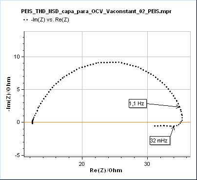
In Fig. 3, the data shown below 32 mHz are due to the change of the polarization resistance of the system with time. As can be seen on the Non-Stationary Distortion (NSD) factor shown in Fig. 4 (See “How to make reliable EIS measurements with your potentiostat or battery cycler” article for a definition of NSD), the impedance data seems to be affected by steady-state and time-variance effects from 1.1 Hz as it is the frequency at which the NSD increases. At 32 mHz the NSD reaches a value as small as 0.58 % and it can be seen in Fig. 3 that such a small value can be representative of the dramatic deformation of the impedance graph.

Figure 4: Non-Stationary Distortion (NSD) of the current response from EIS measurements shown in Fig. 3. Below 1.1 Hz the NSD starts increasing.

How can I correct the effects of time-variance on my EIS measurements ?

One easy way to solve this issue is to use the analysis tool in the EC-Lab^® potentiostat software called Z Inst, which implements a method discovered by Z. Stoynov and B. Savoya [1]. The basic steps of this method are the following:

1. Several impedance graphs are acquired sequentially on a system that changes with time (Fig. 5a).
2. The impedance data are plotted as a function of time (Fig. 5b).
3. The data at the same frequencies are connected and interpolated
4. We obtain an impedance surface
5. By choosing cross-sections of this tunnel we can have instantaneous impedance data (Figs. 5c and d).

Figure 5: a) Nyquist representation of successive impedance graphs of a corroding electrode and b) corresponding 3D representation as a function of time, c) Nyquist representation of instantaneous impedance obtained by the “Z Inst” tool with 20 cross sections and d) corresponding 3D representation as a function of time

The impedance graphs shown in Figs. 5c and d can be considered to have been corrected from the time variance and the change of polarization resistance of the corroding electrode. ZFit can be used to determine all the relevant parameters such as the double-layer capacitance $C_{\mathrm{dl}}$, the charge transfer $R_{\mathrm{ct}}$ and the polarization $R_{\mathrm{p}}$ which is the limit at low frequencies. It should be noted that most of the impedance graphs have an inductive part at low frequencies, which shows that the reduction reaction of protons involves an adsorption step [2].

References

1. Z. Stoynov, B. Savoya, J. Electroanal. Chem. 112 (1980) p. 157
2. J.-P. Diard, P. Landaud, B. Le Gorrec, C. Montella, J. Electroanal. Chem. 255 (1988) p. 1

Further information

Application notes

EIS stationarity – Electrochemistry, Battery & Corrosion – Application Note 55

EIS Quality Indicators: THD, NSD & NSR – Electrochemistry, Battery & Corrosion – Application Note 64

EIS Quality Indicators THD – Electrochemistry, Battery & Corrosion – Application Note 65

White paper

Studying batteries with Electrochemical Impedance Spectroscopy – Electrochemistry & Battery

Literature

http://dx.doi.org/10.5599/jese.725