

THD: parameters affecting its value & comparison with other methods of linearity assessment Battery & Corrosion – Application Note 65
Latest updated: April 14, 2026Abstract
This Application Note develops some aspects of the Total Harmonic Distortion as an indicator of EIS quality, available since EC-Lab® v11.20 as EIS QI™. After presenting the main factors affecting the THD, a comparison with other methods of non-linearity assessment, namely the Lissajous plot, Kramers-Kronig transform, and the model-based method, is presented.
Introduction
EIS QI™ are quality indicators introduced in EC-Lab® v11.20 and described in [1]:
- Total Harmonic Distortion (THD)
- Non-Stationary Distortion (NSD)
- Noise to Signal Ratio (NSR)
The THD is used to quantify the distortion of the response of a system, which can be used to characterize its linearity.
Other methods have been proposed for this purpose:
- Lissajous plot
- Kramers-Kronig (KK) transform
- Model-based method.
In this note, we will first give further details about non-linearity and the THD indicator and secondly give a few comparison elements with other non-linearity indicators, based on results obtained on BioLogic Test Box-3.
Parameters Affecting The THD
As seen in [1], THD is an indicator that quantifies the distortion of input and output signals by measuring the higher harmonics amplitude and dividing it by the amplitude of the fundamental frequency. Hence, the first factor affecting THD is the voltage amplitude of the input signal. For a non-linear system, the higher the voltage amplitude, the more non-linear the response of this system will be.
In this part we will present the other factors affecting the THD. As the behaviour of an electrochemical system is not easy to control, the system that is under study is an electrical circuit that composes the Test Box-3 #3. This electrical circuit mimics the behaviour of an electrode that corrodes and then passivates.
The steady-state I vs. E curve is shown in Fig. 1.

Figure 1: Steady-state I vs. E response of the electrical circuit of Test Box-3 #3.

We can see that this system is typically non-linear as its I vs. E curve does not follow a linear law. However, it is composed of linear segments. We can also distinguish 3 different operational points: Edc1, Edc2 and Edc3.
Edc1: Linear Behaviour
It can be noted that at Edc1, the system is linear over a certain potential range roughly between 0 and 0.5 V. This can be verified in Fig. 2, which shows the impedance measurements performed around Edc1 with increasing voltage amplitudes (Fig. 2a) and the corresponding THD of the current (THD I) (Fig. 2b).
As can be seen in Fig. 2a, whatever the amplitude, the Nyquist diagrams are all superimposed and in Fig. 2b, it can be seen that THD I is not over 2%. The highest values of THD I are only due to signal noise related to the use of a very small amplitude (5 mV) as was also shown in [1].
a)

b)
Figure 2: a) Nyquist diagrams and b) corresponding THD I of EIS measurements performed on Test Box-3 #3 at Edc1 = 0.3 V using increasing amplitudes: 5, 10, 15, 20, 30, 40 mV. Frequency range: 100 kHz – 1 Hz.

Edc2: Non-Linear Behaviour 1
If now we set a DC voltage at a point where the I vs. E curve is not linear we will obtain the results shown in Fig. 3.
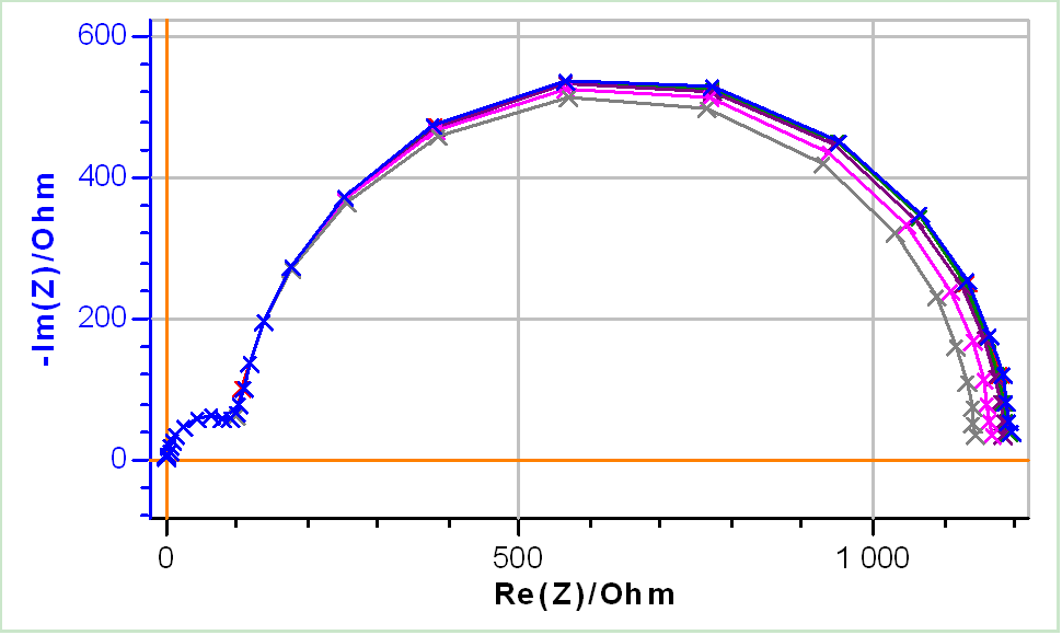
As the amplitude increases, the Nyquist diagrams change, especially at the lower frequencies (Figs. 3a and 3b). This shows that the system, at this particular DC voltage, is not linear. Figure 3c shows the THD I corresponding to the results shown in Figs. 3a and b as a function of the frequency.
It can be seen that the linearity depends on the frequency. For each amplitude, the THD I starts to increase below ca. 100 Hz to reach a plateau at ca. 10 Hz. It can also be seen that it depends on the amplitude of the input modulation when the system is non-linear.
At 5 and 10 mV, the system can be considered to behave linearly because the THD I is below 5% at all frequencies. This is confirmed by Figs. 3a and 3b where the impedance data for these two amplitudes are similar.
a)
b)

c)

Figure 3: a) Nyquist diagrams with b) a close-up on the low frequency values and c) corresponding THD I of EIS measurements performed on Test Box-3 #3 at Edc2 = 0.51 V using increasing amplitudes: 5, 10, 15, 20, 30, 40 mV. Frequency range: 100 kHz – 1 Hz.
Above 10 mV the THD I starts to reach 5% at the lowest frequency (1 Hz). This is confirmed in Fig. 3b where the impedance values are further from each other. At 1 Hz, a THD I difference of 14% (Fig. 3c) produces an impedance modulus difference of 4.2% (Fig. 3b).
Edc3: Non-Linear Behaviour 2
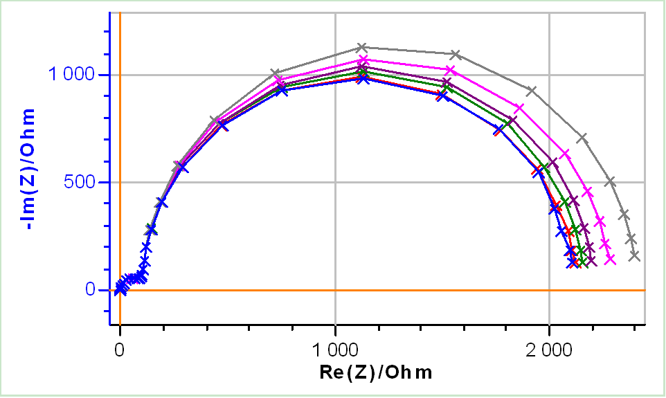
If we now set the DC voltage at Edc3 = 1.07 V, we will obtain the results shown in Fig. 4.
a)
b)
c)
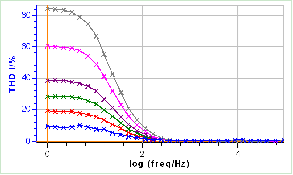
Figure 4: a) Nyquist diagrams with b) a close-up on the low frequency values and c) corresponding THD I of EIS measurements performed on Test Box-3 #3 at Edc3 = 1.07 V using increasing amplitudes: 5, 10, 15, 20, 30, 40 mV. Frequency range: 100 kHz – 1 Hz.
By setting the DC voltage just on the left of the apex of the DC curve, it can be seen that the system has a much more non-linear behaviour. In Figs. 4a and 4b it can be seen that for the same amplitude values as Figs. 2 and 3, the difference in shape of the Nyquist diagrams is much more important. Figure 4c shows that all the chosen amplitudes induce, under a frequency of around 100 Hz, a non-linear behaviour of the system.
One can notice that if we only take impedance data from high frequencies to 100 Hz (log(100) = 2 in Fig. 4c)), then all amplitudes are correct and the system does not behave non-linearly. Increasing the amplitudes in this case increases the low frequency impedance modulus. At 1 Hz a THD I difference of 75% (Fig. 4c) produces an impedance modulus difference of around 14% (Fig. 4b).
Summary
The steady-state I vs. E curve of a system can be used to estimate if a system is intrinsically linear or non-linear in steady-state conditions.
The THD indicator of the response of a system submitted to a sinusoidal modulation around a steady-state value can be used to quantify the dynamic linearity of the system.
The THD (ie the distortion of the response) depends on:
- The amplitude of the input signal.
- The steady-state voltage, that is to say the point along the steady-state I vs. E characteristic.
- The frequency. Generally, in electrochemical systems with large double-layer capacitances, non-linearities appear at lower frequencies.
Comparison With Other Non-Linearity Indicators
In this part we will compare the THD indicator with other ways to estimate the non-linearity of the system. The pros and cons of each method will be shown. We chose three methods: the Lissajous plot, the Kramers-Kronig (KK) relationships and the use of measurement models. The considered methods are those typically used in electrochemistry and EIS studies. Other methods based on neural networks, Kalman filters and other algorithms are not considered here.
Note that the simplest method to test linearity is to perform EIS measurements at various amplitudes and see if the impedance data change with the amplitude. The main drawback is that this is time-consuming.
Lissajous Plot
The Lissajous plot consists of plotting the real time or dynamic E(t) (or I(t)) vs. I(t) (or E(t)) curve corresponding to one frequency EIS measurement. If this curve is elliptical, then it means the system behaves linearly. If the ellipse starts to deform to the shape of the steady-state E (or I) vs. I (or E) curve then the system behaves non-linearly.
Figure 5 shows the simulated Lissajous plot corresponding to the impedance data shown in Fig. 4a at 1 Hz (ie. the lowest frequency).
Each Lissajous curve is plotted around the steady-state I vs. E curve.

Figure 5: Lissajous plots of the data shown in Fig. 4a) at 1 Hz using increasing amplitudes: 5, 10, 15, 20, 30, 40 mV.
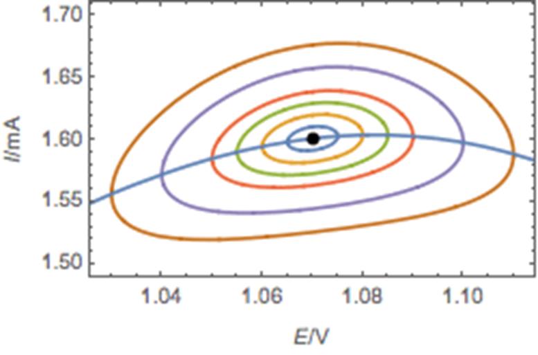
Whereas it is clear for the three larger amplitudes that the shape of the Lissajous curve is not elliptical, it is less obvious for the three lower amplitudes. Conversely, the THD indicator leaves no ambiguity concerning the non-linearity of the system as can be seen in Fig. 4c: at the lowest amplitude and 1 Hz the THD is around 10%. Lissajous is a qualitative, visual tool which is as much an advantage as a drawback.
Another drawback can be seen when considering data and information compacity. In Lissajous, a whole I vs. E curve with enough definition (say 20 data points) is needed at each frequency, whereas for THD, the same information is given by only one data point for each frequency.
Kramers-Kronig
Using the KK transform, the real part of the impedance can be calculated for a causal, stable, linear, time invariant and finite system for f → 0 and f → +∞, using the change in its imaginary part as a function of the frequency. Alternatively, the imaginary part of the impedance can be calculated when the evolution of its real part is known [2-6]. When the impedance of an electrode reaction is measured, it is possible to calculate the imaginary part using experimental values for the real part and calculate the real part using experimental values for the imaginary part. Comparing calculated impedance ZKK with the experimental impedance Z is a useful tool to check the linearity of the impedance measurement with respect to the conditions of applicability of KK transform.
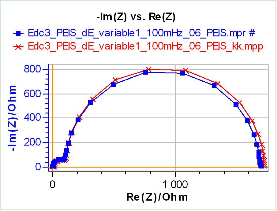
Figure 6a shows the impedance data obtained using the same parameters as in Fig. 4a, only using the largest amplitude (40 mV) and decreasing the lower frequency to 100 mHz, and the corresponding KK transform. Both look very similar, as it is confirmed by Fig. 6b, which shows the differences between these curves in terms of percentage of impedance modulus and of phase degree, as a function of the frequency. The difference or error does not go over 5% for the impedance modulus and below -2 deg for the phase.
Relying on KK transform only, one might want to say that the system is causal, stable, linear, time invariant and finite. But, even though THD goes up to 80% for this data set, KK transform cannot be used to show the non-linearity of the system. As pointed out by Macdonald in [10] “if an electrochemical system obeys the linearity, causality, and stability conditions the impedance data will transform correctly according to the K-K relations. However, the opposite apparently is not true. In other terms, the fact that KK transforms the impedance data correctly cannot lead to any conclusion concerning the system. Another drawback of the KK transform is that it requires the data to be complete, that is to say to start and finish with Re(Z) = 0. This is why Fig. 6a contains data at frequencies down to 100 mHz, instead of data shown in Fig. 4a, which could not be used for KK transform.
a)
b)

Figure 6: a) Nyquist impedance graph of Test Box-3 #3 at Edc3 = 1.07 V using an amplitude of 40 mV (▪) and corresponding KK transform (×). b) Difference of the impedance modulus in % (▪) and the phase in degrees (×) between the experimental data and the KK transform.
Model-Based Method
As was described in [7-9], one way to ensure that EIS data are consistent with KK relations, in other terms that the system under study is causal, stable, linear, time invariant and finite, is to analyze the data using what is called a Voigt circuit. As was already described in the application note about Discrete Relaxation Times (DRT) transformation [11] a Voigt circuit is composed of a series of n R/C circuits.
An R/C circuit is linear and n R/C circuits in series also constitutes a linear system. If impedance data can be fitted using a Voigt circuit it proves they are consistent with KK transform and are resulting from a linear response of the system. Let us consider now the data shown in Fig. 4a. One can use the following equivalent circuit to fit the data: R1/C1 + R2/C2. The results of the fitting procedure using Z Fit without weighing, with Randomize+Simplex minimization method are given in Tab. I for each amplitude. Figure 7 shows the impedance graph for the largest amplitude for which THD reaches a maximum of more than 80% and the corresponding fitting data.
Table I: Parameter values resulting from fitting of data shown in Fig. 4a using Z Fit and R1/C1 + R2/C2 equivalent circuit, for each amplitude.
| δE/mV | R1/Ω | C1/µF | R2/Ω | C2/µF |
|---|---|---|---|---|
| 5 | 105.6 | 47.6 | 1996 | 4.92 |
| 10 | 105.8 | 47.8 | 2008 | 4.95 |
| 15 | 105.0 | 47.5 | 2050 | 4.92 |
| 20 | 105.5 | 47.5 | 2091 | 4.92 |
| 30 | 106.1 | 47.7 | 2171 | 4.95 |
| 40 | 106.5 | 47.7 | 2290 | 4.96 |

Figure 7: Nyquist impedance graph of Test Box-#3 at Edc3 = 1.07 V using an amplitude of 40 mV (▪) and the corresponding fitting curve using R1/C1+R2/.
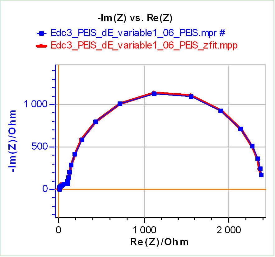
The results in Tab. I and Fig. 7 show that data can be fitted by a Voigt equivalent circuit with two R/C in series. The conclusions drawn from the THD results shown in Fig. 4c and even from the corresponding Lissajous plots shown in Fig. 5 tell us that the system response is non-linear at all amplitudes.
Consequently, the measurement model method appears to be failing in this case in the sense that we can only deduce something from the system if the method fails, not if it succeeds. In this regard it has the same drawback as the KK transform.
Summary
Table II below summaries the various pros and cons of the different methods.
Table II: Comparison of the main methods for linearity estimation used in electrochemistry.
| + | – | |
|---|---|---|
| EIS at various amplitudes | Easy to implement and understand | Time-consuming |
| THD | Quantitative information; 1 data point/frequency | Requires theoretical understanding |
| Lissajous | Visual and easy to apprehend | Only gives qualititative information; requires many data at each frequency |
| Kramers-Kronig | Test the general validity of the data (not only linearity) | Only useful if it fails; cannot be used when Nyquist data are incomplete |
| Meas. Model | Easy to implement | Only useful if it fails |
Conclusion
In this application note, we presented the main factors affecting THD: input amplitude, frequency and operating voltage. Each aspect was illustrated by results performed on a BioLogic Test Box-3. In a second part, we considered three other methods of linearity assessment and compared them with the THD indicator.
Data files can be found in :
C:\Users\xxx\Documents\EC-Lab\Data\Samples\EIS\AN65_
References
1) Application Note #64 “Introducing EC-Lab® EIS quality indicators: THD, NSD and NSR.”
2) Application Note #15 “Two questions about Kramers-Kronig transformations”
3) V. A. Tyagay, G. Y. Kolbasov, Elektrokhimiya, 8 (1972) 59.
4) R. L. V. Meirhaeghe, E. C. Dutoit, F. Cardon, W. P Gomes, Electrochim. Acta, 21 (1976), 39.
5) J.-P. Diard, P. Landaud, J.-M. Le Canut, B. Le Gorrec, C. Montella, Electrochim. Acta, 39 (1994) 2585.
6) A. Sadkowski, M. Dolata, J.-P. Diard, J. Electrochem. Soc., 151 (1) E20.
7) P. Agarwal, M. Orazem, L. Garcia-Rubio, J. Electrochem. Soc., 139 7 (1992) 1917
8) P. Agarwal, M. Orazem, L. Garcia-Rubio, J. Electrochem. Soc., 142 12 (1995) 4159
9) P. Shukla, M. Orazem, O. Crisalle, Electrochim. Acta, 49 (2004) 2881
10) M. Urquidi-Macdonald, D. Macdonald, Electrochim Acta, 35, 10 (1990) 1559
11) Application Note #60 “Distribution of Relaxation Times (DRT): an introduction”
Revised in 07/2018


