

How to access electric variables in EC-Lab®
Latest updated: November 6, 2025The conductivity of the materials used in batteries is one of the critical variables to be studied, especially for All-Solid-State Batteries (ASSB). A low conductivity means high resistance. This can lead to heat generation and thus to a rapid increase in the battery temperature during operation, which can initiate thermal runaway (see: Battery science: Interactive glossary of terms – Thermal runaway).
Electrochemical Impedance Spectroscopy (EIS) is a powerful analytical tool for investigating the electrical properties of materials. It can provide quantitative information on many electrical parameters, such as conductivity, permittivity, resistivity, etc. Over the last couple of decades, it has been widely applied to the study of solid-state devices.
Several electrical variables have been implemented in EC-Lab® V11.40 and higher, calculated from the real and imaginary parts of the impedance (Table 1). For some systems, electrical variables can be determined accurately without fitting with an equivalent circuit, allowing direct analysis and saving time in many cases. The ε0 and k parameters correspond to the vacuum permittivity and the cell constant respectively and ω is the angular frequency.
Table 1: List of electrical variables in EC-Lab®.
| Electrical variable | Description | Formula |
|---|---|---|
| $$\text{Re}(conductivity)$$ | Real part of the complex conductivity | $$k\frac{\text{Re}(Z)}{\left|Z\right|^2}$$ |
| $$\text{Im}(conductivity)$$ | Imaginary part of the complex conductivity | $$-k\frac{\text{Im}(Z)}{\left|Z\right|^2}$$ |
| $$\text{Re}(resistivity)$$ | Real part of the complex resistivity | $$\frac{\text{Re}(Z)}{k}$$ |
| $$\text{Im}(resistivity)$$ | Imaginary part of the complex resistivity | $$-\frac{\text{Im}(Z)}{k}$$ |
| $$\text{Re}(C)$$ | Real part of the complex capacitance | $$\frac{-\text{Im}(Z)}{\omega\left|Z\right|^2}$$ |
| $$\text{Im}(C)$$ | Imaginary part of the complex capacitance | $$\frac{\text{Re}(Z)}{\omega\left|Z\right|^2}$$ |
| $$\text{Re}(M)$$ | Real part of the complex modulus | $$-\omega\frac{\varepsilon_0}{k}\text{Im}(Z)$$ |
| $$\text{Im}(M)$$ | Imaginary part of the complex modulus | $$\omega\frac{\varepsilon_0}{k}\text{Re}(Z)$$ |
| $$\text{Re}(permittivity)$$ | The real part of the complex permittivity | $$-\frac{k\text{Re}(Z)}{{\varepsilon_0\omega\left|Z\right|}^2}$$ |
| $$\text{Im}(permittivity)$$ | Imaginary part of the complex permittivity | $$\frac{k\text{Im}(Z)}{{\varepsilon_0\omega\left|Z\right|}^2}$$ |
| $$Tan(Delta)$$ | Dielectric loss factor | $$-\frac{\text{Re}(Z)}{\text{Im}(Z)}$$ |
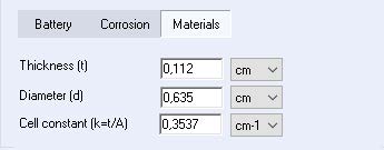
The cell constant (k) can be added directly in the material section of the cell characteristic tab, or it can be calculated by EC-Lab® when the thickness and diameter of the sample are specified (see Figure 1).

Figure 1: Cell constant value (k) obtained automatically in the cell characteristic tab on the EC-Lab® Software.
The electrical variable as a function of frequency can be plotted by selecting the desired variable on the file selection window (Figure 2).

Figure. 2: File selection window
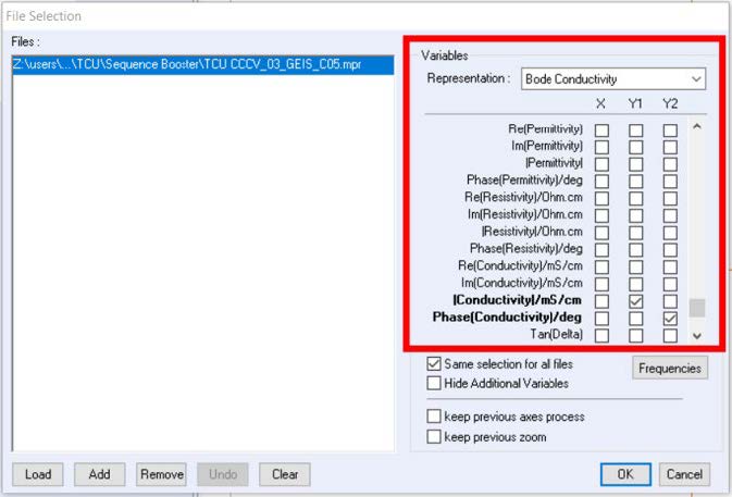
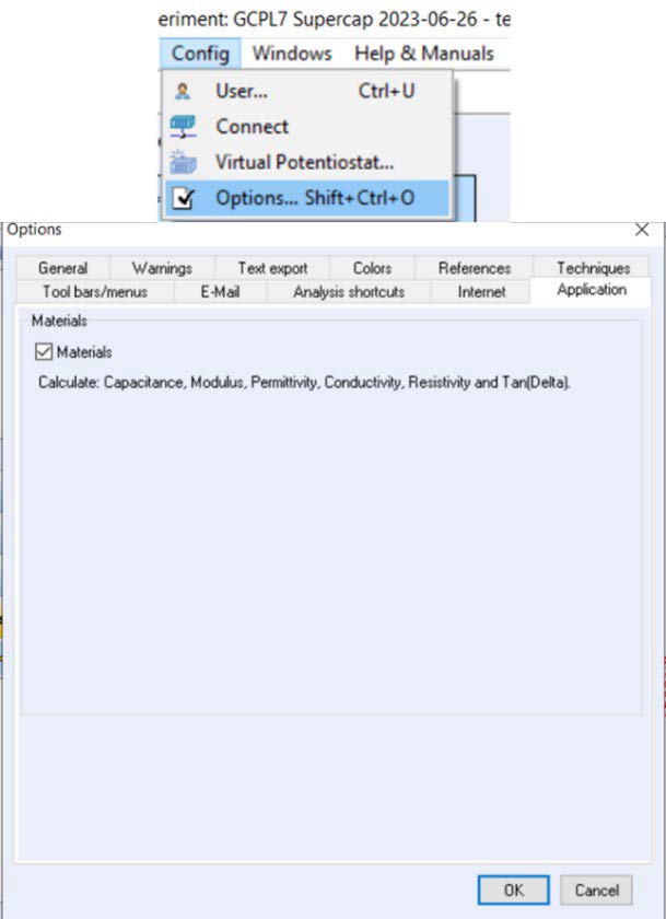
If the variables are not visible on the file selection window, the Materials checkbox must be activated in the Config menu → Options → Application section (Figure 3).

Figure 3: Activation of the materials checkbox
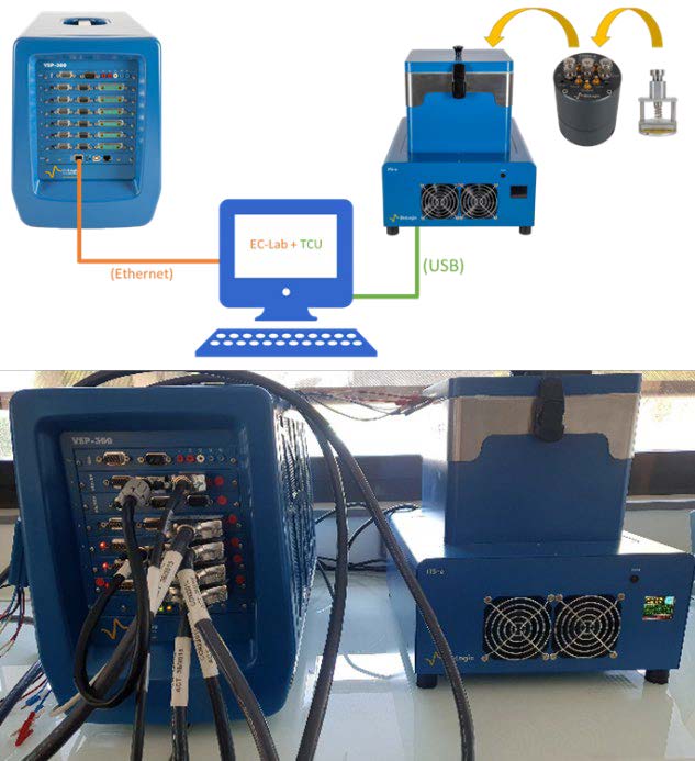
The temperature-dependent electrical measurements can be determined using a BioLogic Premium potentiostat/galvanostat (up to 11 MHz with standard cable) coupled with an Intermediate Temperature System (ITS-e) to control the temperature. A controlled Environment Sample Holder (CESH-e) can be used to hold the solid sample, apply pressure, and/or control the sample’s atmosphere. The CESH-e can be placed in the ITS-e and connected to the potentiostat using the Temperature Control Unit (TCU) interface to communicate with EC-Lab® Software. Figure 4 shows a picture of an experimental setup that can be used for the determination of electrical variables.

Figure 4: CESH-e into the ITS-e unit connected to a VSP 300.
The high-frequency region is crucial for the analysis of electrical variables, therefore, compensation using EC-Lab® software is necessary for the electrochemical impedance measurements. If not done, additional parasitic elements (i.e., capacitance, inductance, or resistance) not directly due to the device under test (DUT) can contribute to the results (For more information about compensation please see: How to correct impedance measurements when using longer cables).
An example of an application using the EC-Lab® electrical variables is shown in Figure 5 for a solid-state electrolyte. Arrhenius plot shows similar values of the ionic conductivity when comparing the conductivity obtained graphically on the high-frequency range of the real part of the complex conductivity to those obtained by fitting an equivalent circuit.

Figure 5: Comparison of Arrhenius plot of the ionic conductivity of a solid-state electrolyte at temperatures between – 40 °C and 10 °C.


