$\small R_\text p = \lim \limits_{f \rightarrow 0} \text{Re} \;Z$. Why?

${I\,vs.\,U}$ steady-state polarisation curve

Consider the electrical circuit R1/C1+R2/C2. In steady-state conditions, the capacitive currents are zero and this circuit is equivalent to the R1+R2 circuit. The potential difference $U$ at the terminals of the circuit through which the current $I$ flows is given by

$$ U=(R_1+R_2) I \Rightarrow I=U/(R_1+R_2) \tag 1$$

In steady-state conditions the slope $p$ of the line $I\, vs. \,U$ is equal to $1/(R_1+R_2)$.

The polarization resistance $R_\text p$, which is, by definition, the inverse $1/p$ of the slope of the line $I\, vs. \,U$, obtained in steady-state conditions (ie at very slow potential scan rates), is given by $R_1+R_2$ (Fig. 1).

Fig. 1 : $I \;vs.\; U$ steady-state polarisation curve of the electrical circuit R1/C2+R2/C2.

This result does not, of course, apply in the case of impedances with a non-real low-frequency limit, such as, for example, capacitors, CPE, or the restricted diffusion element M.

Nyquist impedance diagram

The impedance of the R1/C1+R2/C2 circuit is given by

$$ Z(f)= \frac{R_1}{1+R_1\,C_1 \,j \;2\, \pi\, f}+\frac{R_2}{1+R_2\,C_2 \,j \;2\, \pi\, f} \tag 2$$

One of its graphs in orthonormal Nyquist’s plane is shown in Fig. 2 and the low frequency limit of the real part, $R_\text{lf}$, is equal to $R_1+R_2$. We can conclude from this example that $ R_\text p = R_\text{lf}$.

A second method in the time domain instead of the frequency domain can be used to explain this result.

Fig. 2: Nyquist impedance diagram of the electrical circuit R1/C2+R2/C2

Response to a Potential Step

The response potential $\delta U(t)$ of circuit R1/C1+R2/C2 to a current step with amplitude $\delta I$ can be calculated by Laplace transform [1]. It is obtained:

$$ \delta U= \left(R_1 \left(1-\exp \left(-{t}/{(R_1 C_1)}\right)\right)+R_2 \left(1-\exp \left(-{t}/(R_2 C_2)\right)\right)\right) \,\delta I \tag  3$$

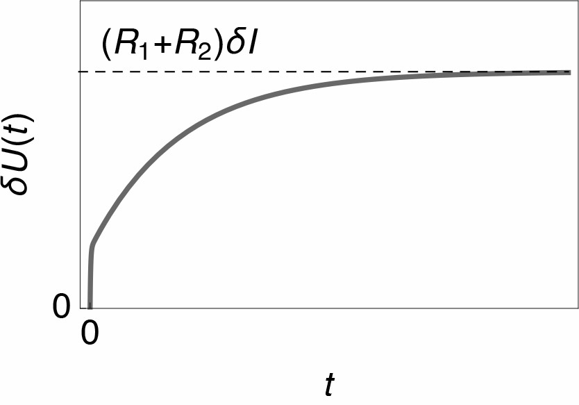
Fig. 3: Sketch of the response of circuit R1/C1+R2/C2 to a current step with amplitude $\delta I$.

The long time limit $\delta U(\infty)$, corresponding to low frequencies, is $(R_1+R_2)\delta I$ and the polarization resistance is given by

$$ R_\text p = \frac{\delta U(\infty)}{\delta I}=R_1+R_2 \tag 4$$

in accordance with the previous result.

Generalization

The final value theorem generalises the result $R_\text p= R_\text{lf}$  [2,3]. It is written

$$\lim \limits_{t \rightarrow +\infty} f(t)=\lim \limits_{s \in \mathbb R,\,s \rightarrow0^+} s\, F(s) \tag 5$$

where $F(s)$ is the Laplace transform of a function of time $f(t)$ and $s$ the Laplace variable. For any time-invariant and stable system with impedance $Z(s)$ submitted to a current step with amplitude $\delta I$ whose Laplace transform is $\delta I/s$ we have

$$\lim \limits_{t \rightarrow +\infty} \delta U(t)=\delta U(\infty) =\lim \limits_{s \in \mathbb R,\,s \rightarrow0^+} s\, \frac{\delta I}{s}\, Z(s)=\delta I \,Z(0) \Rightarrow \tag 6$$

$$R_\text p=\frac{\delta U(\infty) }{\delta I}=Z(0)  \tag 7$$

[1] BioLogic Application note #50. Math reminder for Electrochemists II. The simplicity of Laplace transform.

[2] Laplace transform in Wikipedia. Accessed:

2021-03-15.

[3] D. A. Harrington and P. v. d. Driessche. Electrochim. Acta, 56, 23 (2011) 8005