

EC-Lab® & BCS-800 with BT-Lab® graphic customization Battery – Application Note 26
Latest updated: April 19, 2024Abstract
The aim of this application note is to demonstrate the power and usefulness of the EC-Lab and EC-Lab Express graphical representations. Applications such as RDE voltammetry and battery discharging are used as examples for creating custom graphs using some of the 24 mathematical functions available in the Graph Properties menu to process the acquired data. With the right graphical presentation, other analysis tools such as wave analysis and linear fit can be utilized to extrapolate critical kinetic parameters.
Introduction
A good graphical representation makes the understanding of the data easier. EC Lab® and EC-Lab® Express software provide a traces processing tool (Fig. 1) which allows the user to customize its own traces.
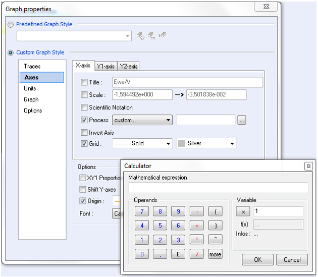
Figure 1: Traces process windows.
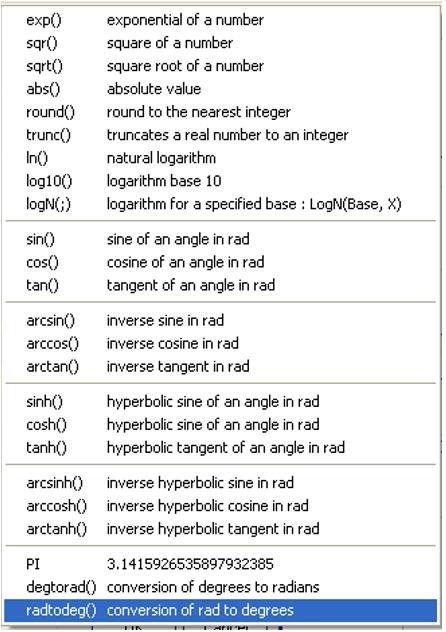
Figure 2: Mathematical functions available in calculator.
24 mathematical functions (Fig. 2) are available (button “more” of the calculator) for writing mathematical expression of X-, Y1- or Y2-axis.
In this application note, some examples of graphic customization are shown in various field of electrochemistry.
RDE Voltammetry Application
The plot log [i/(ilim – i)] = E could be required in order to determine the standard potential and the number of electron involved in the redox process under stationary condition and for Nernstian system. Consequently, this feature is used in Rotating Disk Electrodes (RDE) voltammetry investigations [1] or in the field of the High Performance Liquid Chromatography (HPLC) with electrochemical detection [2].
In this context, a solution of K4Fe(CN)6 at 10 mmol·L-1 is studied by RDE voltammetry with RRDE-3A in aqueous electrolyte with KCl (0.1 mol·L-1) as supporting salt. Three-electrodes set-up is used and constituted as follows:
- platinum electrode (surface electrode A = 0.126 cm²) as working electrode,
- Ag/AgCl electrode as reference electrode,
- alloy wire as counter electrode.
Scan rate and rotating rate are of 50 mV·s-1 and 500 rpm, respectively.
The corresponding voltammogram is shown in Fig. 3 and the “Wave Analysis” tool gives the ilim equal to 766 µA and E1/2 = 223 mV vs. Ag/AgCl.

Figure 3: Steady-state curves [K4Fe(CN)6] = 10 mM H2O + KCl (0.1 mol.L-1) for u = 50 mV·s-1 and Ω = 500 rpm (top) and “Wave Analysis” result (bottom).
Current for Nernstian system under stationary condition are given by the following relationship
$$i_f=\frac{nF\left[X\right]_{init}\ \mathrm{exp}{\left(\frac{nF}{RT}\left(E-E^0\right)\right)}}{1+\delta\ \mathrm{exp}{\frac{\left(\frac{nF}{RT}\left(E-E^0\right)\right)}{D}}} \tag{1}$$
where n is the number of electron involved in the process, F is the Faraday number, [X]init is the initial concentration of X in solution, R is the Boltzmann number, T is the temperature and E0 is the standard potential, d is the thickness of the diffusion layer and D the diffusion constant.
$$\mathrm{log}\left[\frac{i}{i_\mathrm{lim} – i}\right] = aE – b \tag{2}$$
$$n=\frac{F}{2.3RTb} \tag{3}$$
$$E_{1/2}=-\frac{b}{a} \tag{4}$$
where ilim is the limiting current, a and b are respectively the slope and y-intercept of the curve.
The resulting graphic is plotted in Fig. 4 and “Line Fit” function gives the following equation:
$\mathrm{log}\ [i/(766 – i)] = 16.2\ E + 3.251$
According the equations (2), (3) and (4), n is equal to 1 (mono-electronic oxidation) and E1/2 is 201 mV vs. Ag/AgCl which is closed to the value determined previously by “Wave Analysis”.
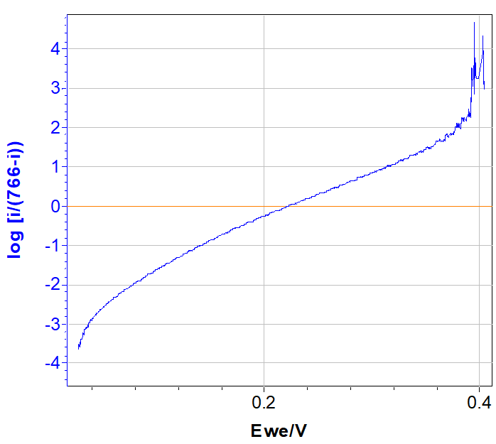
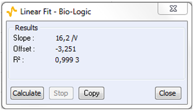
Figure 4: log(i/(ilim – i)) = E plotted (top) and “Line Fit” result (bottom).
On the other hand, this graphical method can be also used as verification method for determining ilim. Indeed, trials with higher (1.05 ilim) or lower (0.95 ilim) ilim exhibit non-linear behavior (Fig. 5).
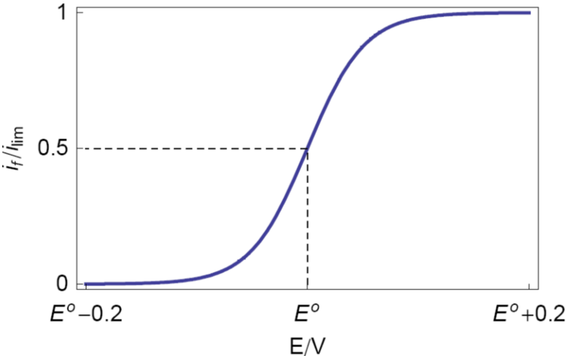

Figure 5: Theoretical steady state voltamogram (top) and logarithmic transform with various ilim (bottom).
Battery Applications
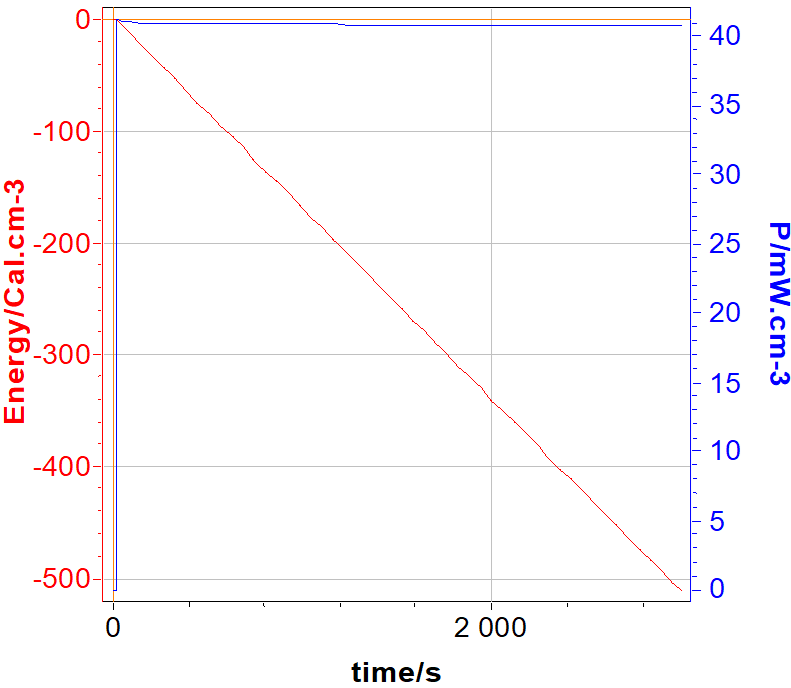
Figure 6: volumic energy (cal·cm-3) and volumic power (W·cm-3) vs. time. The volume of the battery is 160 cm3.
In spite of the official unit of energy is the Joule (W.s), the calorie (1 J = 4.18 cal.) is also used as energy unit in the medical area, and particularly, for implantable battery. In this context, the volumic energy of battery in calorie is plotted vs. time
On the other hand, for information, the volumic power is also plotted in Fig. 6 on the Y2-axis.
In this context, discharge (GCPL technique) of LiFePO4 battery is carried out with a 8 A booster connected to a VMP3.
N.B.: To have power values, power must be ticked in the “Advanced Setting” before starting measurement.
EIS Applications
The impedance is certainly the field of electrochemistry where graphical methods are the most useful to better interpret and evaluate data [3,4] , for example, the determination of the a parameter of Constant Phase Element (CPE).
Investigations are performed with VSP instrument driven by EC-Lab® software in a solution of HCl (0.1 M). The three-electrode set-up is used with:
– rotating Disk Electrode (RDE) of iron as working electrode with a surface area of 3.14 mm²,
– platinum wire as counter electrode,
– saturated Calomel Electrode (SCE) as reference electrode.
Experiments are carried out at 800 rpm as rotation speed of the electrode.
Resulting Nyquist plot is shown in Fig. 7.
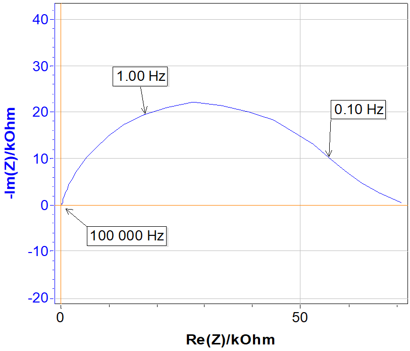
Figure 7: Nyquist plot.
Let us consider the equivalent circuit shown in Fig. 8 which is valid in the high frequency area.

Figure 8: Equivalent circuit R in series with a CPE, noted Q.
The corresponding impedance is given by:
$$Z=Z_Q=\frac{1}{Q(i2\pi f)^\alpha} \tag{6}$$
If RΩ = 0, the magnitude and imaginary part of the impedance are written [5,6] :
$$|Z|=\frac{1}{Q(2\pi f)^\alpha} \Rightarrow \mathrm{log}|Z|=-\alpha \mathrm{log}{f}-\mathrm{log}(Q(2\pi )^\alpha) \tag{7}$$
$$\mathrm{Im}\ Z=-\frac{sin(\alpha\pi/2)}{Q(2\pi f)^\alpha}\ \Rightarrow\mathrm{log}|\mathrm{Im}\ {Z}|=-\alpha\ \mathrm{log}f-\mathrm{log}{\left(\frac{Q(2\pi)^\alpha}{sin(\alpha\pi/2)}\right)} \tag{8}$$
Therefore plotting log|Z| or log|ImZ| vs. log|f| yields to a straight line with a slope given by -α (Fig. 9) at high frequency.
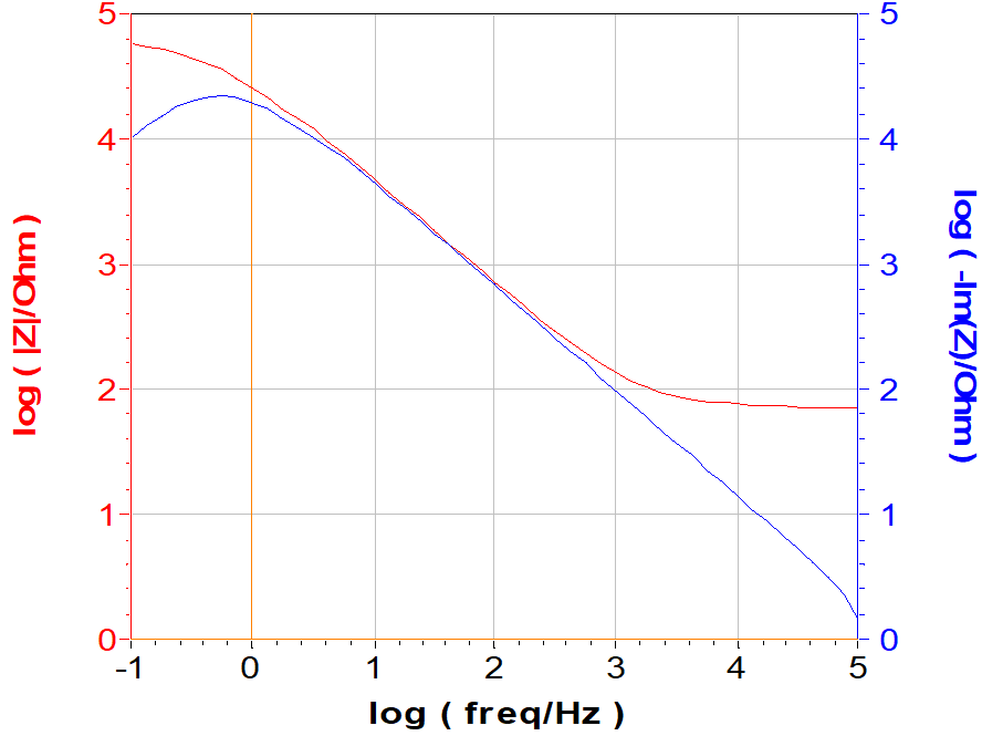
Figure 9: Bode representation and log(-Im Z) vs. log frequency.
If RΩ ≠ 0, the impedance is given by:
$$Z=R_\Omega+\frac{1}{Q(i2\pi f)^\alpha} \tag{9}$$
and the magnitude is written:
$$|Z_Q|=\sqrt{R^2+\frac{1}{Q^2(2\pi f)^{2\alpha}}+ \frac{2R\mathrm{cos}(\alpha \pi/2)}{Q(2\pi f)^{\alpha}}} \\
\Rightarrow \mathrm{log}|Z_Q|= \frac{1}{2}\mathrm{log}\left(R^2+\frac{1}{Q^2(2\pi f)^{2\alpha}}+ \frac{2R\mathrm{cos}(\alpha \pi/2)}{Q(2\pi f)^{\alpha}}\right) \tag{10}$$
while the expression of the imaginary part of the impedance remains unchanged. Only the plot of log|Im Z| vs. log f yield to a straight line for RΩ ≠ 0.
The a coming from the Line Fit of the two representations are recorded in Tab. I. The comparison of the two values determined by the two graphical methods and the values determined in Application Note #21 [7] are in good agreement.
Table I: Summary of the α parameters.
| log (-Im Z) | Bode | Z Fit from [7] | |
|---|---|---|---|
| α | 0.8397 | 0.8113 | 0.8407 |
Conclusion
Examples given in this note show the capabilities of the EC-Lab® graphic tool. But they are not exhaustive and others customization are also available in order to meet the need of each user.
This application note can be completed by the technical notes #22 [8] and #23 [9] .
References
1) B. Trémillon, G. Durand, Électrochimie. Caractéristiques courant-potentiel: théorie (partie 1), Techniques de l’ingénieur, Paris, (1993).
2) A. Aoki, T. Matsue, I. Uchida, Anal. Chem., 64 (1992) 44.
3) M. E. Orazem, N. Pébère, B. Tribollet, J. Electrochem. Soc., 153 (2006) B129.
4) M. J. Rodiguez-Presa, R. I. Tucceri, M. I., Florit, D. Posadas, J. Electroanal. Chem., 502 (2001) 82.
5) J.-P. Diard, B. Le Gorrec, C. Montella, Exercices de cinétique électrochimique. II. Méthode d’impédance, Hermann, Paris, (2005).
6) J.-P. Diard, B. Le Gorrec, C. Montella, Handbook of EIS, (2017).
7) Application Note #21, “Measurements of the Double Layer Capacitance”
8) Technical Note #22, “Graphic Properties, Part I: Graph Style Definition”
9) Technical Notes #23, “Graphic Properties, Part II: Graph Representation Definition”
Revised in 07/2018


