

Measurements of double layer capacitance Battery & Corrosion – Application Note 21
Latest updated: November 14, 2023Abstract
In this application note, the electrical double layer of an iron electrode in acidic media is investigated. The capacitance is determined by both Electrochemical Impedance Spectroscopy (EIS) and Cyclic Voltammetry (CV) techniques. For the EIS data, the ZFit and the pseudo capacitance tools are used to automate the capacitance calculation from an R/Q circuit.
Introduction
All electrochemical processes take place at the electrode/electrolyte interface, i.e. the electrical double layer (Figure 1). Different models of this layer were stated by Helmholtz, Gouy-Chapman, Stern, or Grahame [1,2].
![Schematic of the electrical double layer according to the Grahame model (adapted from [2]).](https://biologic.net/wp-content/uploads/2019/08/an21f1.jpg)
Figure 1: Schematic of the electrical double layer according to the Grahame model (adapted from [2]). IHP: Inner Helmholtz Plane, OHP: Outer Helmholtz Plane. A: Electrode with an excess of negative charge; B: Localization of the charge in excess; C: Potential change versus distance towards the electrode /electrolyte interface.
The structure of the double layer is similar to an electrical condenser constituted by two charged areas separated by a dielectric. The dielectric thickness corresponds to the ionic radius, i.e. 50 nm.
In this note, the electrical double layer of the iron electrode in acidic conditions is investigated. For this purpose, two techniques are used to determine the value of the capacitance: the Electrochemical Impedance Spectroscopy (EIS) and Cyclic Voltammetry (CV).
Experimental Conditions
Investigations are performed by the VSP instrument driven by EC-Lab® software in a solution of HCl (0.1 M). The three-electrode set-up is used with:
- a Rotating Disk Electrode (RDE) of iron as a working electrode with a surface area of 3.14 mm2,
- a platinum wire as a counter electrode,
- a Saturated Calomel Electrode (SCE) as a reference electrode.
For both techniques, experiments are carried out at the rotation speed of the electrode: Ω = 800 rpm (rotations per minute). For the CV experiment, the scan rate is 40 mV·s-1.
Data analysis for both techniques is also computed by EC-Lab® software.
Impedance Theory
The equivalent circuit, described in Figure 2, with a capacitance and a resistance in parallel and an additional resistance corresponding to the ohmic drop (R1+C/R2) should be a good model for the double layer. In this case, the resulting Nyquist diagram is close to a perfect semi-circle (Figure 2). However, for real systems, this is hardly ever the case. That’s why a constant phase element (CPE), noted Q in Figure 3, is introduced and used instead of the capacitance C in the R1+Q/R2 equivalent circuit [3,4]. Consequently, the resulting Nyquist diagram (Figure 3) corresponds to a depressed semi-circle in its upper-part.
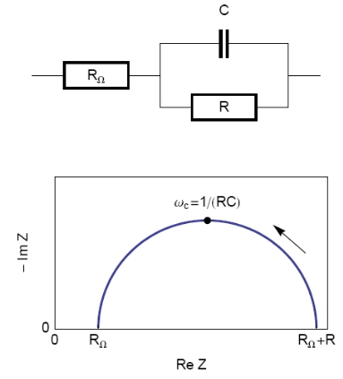
Figure 2: Equivalent electrical circuit RΩ+R/C (top) and corresponding Nyquist impedance diagram (bottom, arrow indicates increasing angular frequencies).
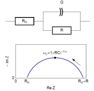
Figure 3: Equivalent electrical circuit RΩ+R/Q (top) and corresponding Nyquist impedance diagram (bottom, arrow indicates increasing angular frequencies).
Then, the analogy between the relationship described in Figs. 1 and 3 leads to Eq. 1. This equation gives the capacitance value at the frequency corresponding to the apex of the Nyquist diagram.
$$C_{\mathrm{dl}} = Q(\omega_c)^{\alpha – 1} \tag{1}$$
Impedance Results and Analysis
The measurements are carried out with potentiostatic EIS (PEIS) techniques at open circuit voltage Eoc in the 100 kHz – 100 mHz frequency range and with a sinus amplitude (Va) of 10 mV. The settings of the impedance investigation are shown in Figure 4.
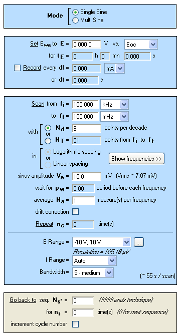
Figure 4: Potentiostatic Impedance “Parameters Settings” window.
The points of the impedance diagram corresponding to lowest frequencies (Re(Z) ≥ 55 kΩ) clearly show that the system drifts with time, because of the time variant condition [5]. Therefore, these points are not taken into consideration (Figure 5).
As explained above, the fit is performed with the R1+R2/Q equivalent circuit (Fig. 6). First of all, the results show that the ohmic drop resistance (R1 = RΩ = 71 Ω) is insignificant before the charge transfer resistance (R2 = Rt = 58 kΩ). Moreover the value of Q is 6.3 µF·sα-1 with α equal to 0.84.
At this point, the capacitance of the system is computed with the “Pseudocapacitance” tool and the value of 5.2 µF is determined for Cdl (Figure 6) [4].
It is possible to load the settings and the data files as PEIS_CPE.mpr in the EC-Lab® Samples, Fundamental Electrochemistry folder.
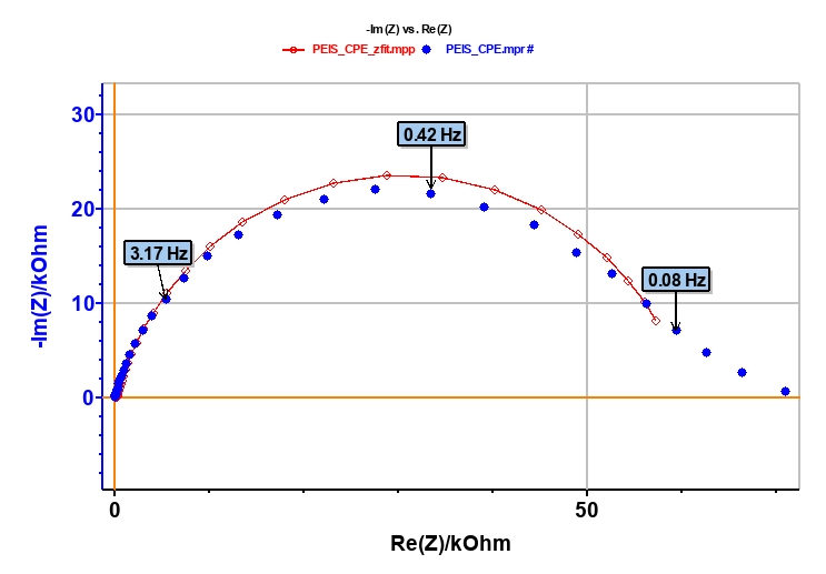
Figure 5: Experimental (blue markers) and fitted (red curve) impedance diagram.
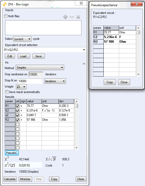
Figure 6: The “ZFit” and “Pseudocapacitance” results.
Cyclic Voltammetry Results And Analysis
Eoc is determined before starting the CV experiment. The value is -0.235 V vs. SCE. The parameters of the CV technique (Figure 7) are chosen accordingly, i.e. in a range of ±15 mV around Eoc with a scan rate of 40 mV·s-1.
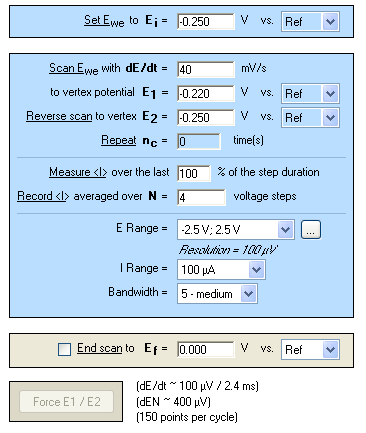
Figure 7: Cyclic Voltammetry “Parameters Settings” window.
As the ohmic drop can be neglected (see previous paragraph), the value of Rp can be determined by calculating the slope of the curve. The Rp values found for forward (Fig. 8) and backward sweeps of the potential are 57 kΩ (= 1/17.673 x 10-6) and 61 kΩ respectively. Note that the Rp values determined by PEIS or CV techniques are in agreement. As the transport of the material does not limit the kinetics of the redox process, the following Eq. 2 is true [2]:
$$R_p = R_t \tag{2}$$
Assuming our system could be modeled by a real capacitance and a resistance in parallel; we can calculate the equations corresponding to the upper and lower part of the curve around the corrosion potential which is equal to Eoc. From these equations, we extrapolated the two current values Ia and Ic corresponding to the corrosion potential for the anodic and the cathodic part of the curve, respectively, and were able to calculate the double layer capacitance with the following equation:
$$\frac{I_a – I_c}{2} = C_{\mathrm{dl}}\frac{\mathrm{d} E}{\mathrm{d} t} \tag{3}$$
Finally, considering the values given in Figure 8 and Eq. 3, the capacitance, Cdl, is 4.3 μF.
It is possible to load the settings and the data files as CV_CPE.mpr in the EC-Lab® Samples folder.
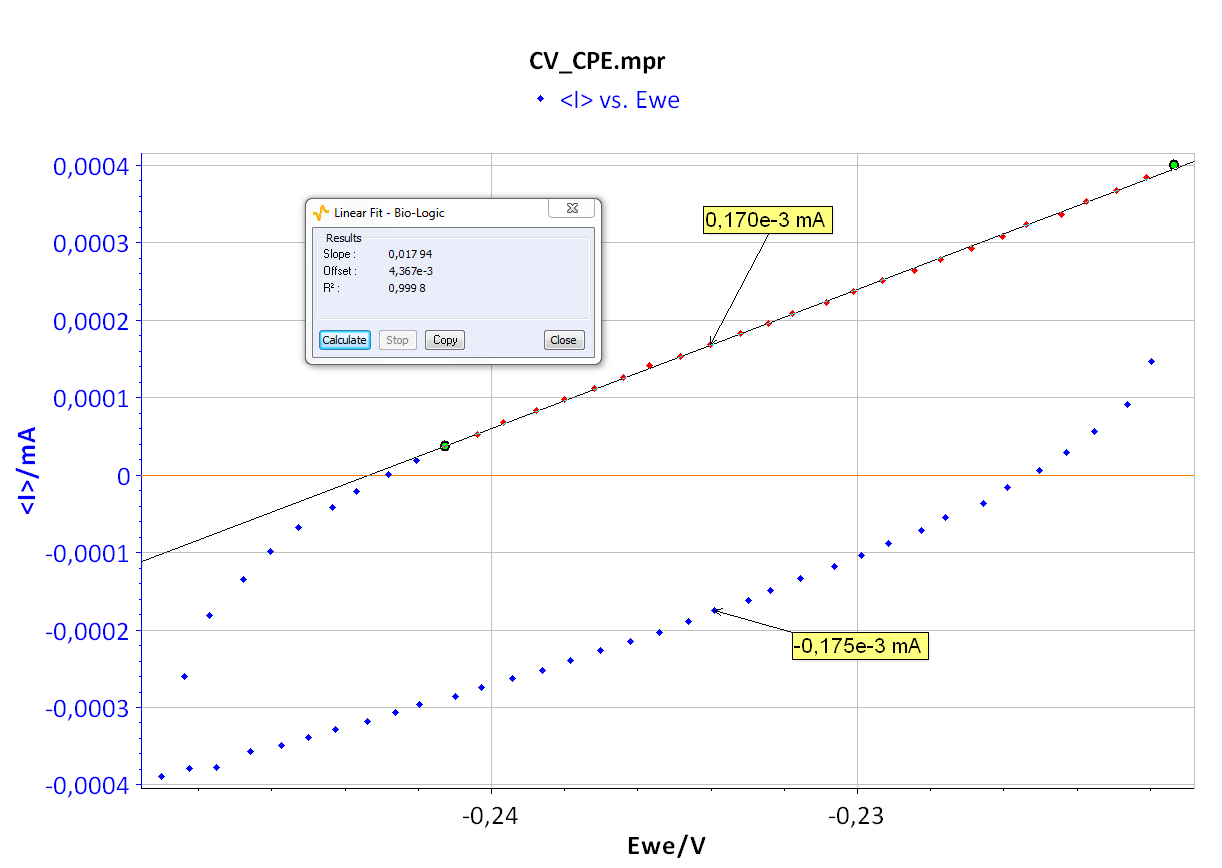
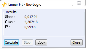
Figure 8: CV curve I vs. EWE for forward and backward voltage scan (top). “Linear Fit” tool for determining Rp (bottom).
It may be of interest to know it is possible to simulate the CV response of a circuit R/Q (Figure 3). For that purpose, the relationship Eq. (4), which expresses the current response of an R/Q circuit to a linear change of potential, is used:
$$I(t)=\frac{v_bt}{R2}+\frac{Qv_bt^{1-\alpha}}{\Gamma(2-\alpha)} \tag{4}$$
where vb is the scan rate of the electrode potential, the Euler gamma function, α the dispersion parameter of the CPE and s the Laplace variable.
Figure 9 shows the experimental data points and the data simulated using Eq. 4. The results of the data fitting on the experimental points gives a value of 8.2 µF·sα-1 with α = 0.841 determined by EIS.
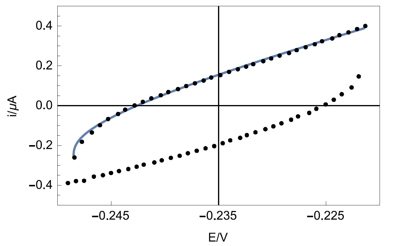
Figure 9: Experimental points (dots) and Simulation (line) of the CV response of circuit R+R/Q (Figure 3) plotted by Mathematica software.
Conclusion
In this note, we have shown how to calculate capacitance values using EIS and CV. Firstly, it was assumed that the double layer was a true capacitance, and secondly it was a constant phase element (CPE). In this case, a pseudo capacitance was calculated and compared to the true capacitance value. The values given by all assumptions and all methods were all of the same order of magnitude.
Table I: Summary
| EIS | CV | ||
|---|---|---|---|
| Cdl Cdl/µF | CPE Q/µF·sα-1 | Cdl Cdl/µF | CPE Q/µF·sα-1 |
| 5.2 | 6.3 | 4.3 | 8.2 |
Data files can be found in:
C:\Users\xxx\Documents\EC-Lab\Data\Samples\Fundamental Electrochemistry\technique_CPE
References
1) A. J. Bard, L. R. Faulkner, Electrochemical methods. Fundamentals and applications, Wiley, Hoboken, (2001).
2) J.-P. Diard, B. Le Gorrec, C. Montella Cinétique électrochimique, Hermann, Paris, (1996).
3) E. Barsoukov, J.R. Macdonald, Impedance Spectroscopy. Theory, experiment and applications., Wiley, Hoboken, (1987).
4) Application Note #20 “Pseudo capacitance calculation”
5) Application Note #55 “Interpretation problems of impedance measurements made on time variant systems”
Revised in 04/2023


