Ohmic Drop Part III: Suitable use of the ZIR techniques (Ohmic drop & ZIR techniques) Battery – Application Note 29

Introduction

As shown in Application note #28 [1], EIS measurements are a good way of determining electrolyte resistance R_Ω (or R_u for uncompensated resistance [2]). R_Ω is defined as the solution resistance between the working electrode and the reference electrode plus any resistances in the working electrode itself, wires, etc. [2, 3].

The EC Lab^® ZFit tool or EC-Lab^® Express software allows the user to calculate this R_Ω value. Nevertheless, the ZFit tool implies that the equivalent electrical circuit is known, which is sometimes not obvious.

The aim of this note is to present the IR determination and compensation by impedance measurement technique (ZIR) and then determine the R_Ω value without using the ZFit tool. A part of this note will be dedicated to enlightening the limits of this technique for some systems.

ZIR techniques

IR determination and compensation by impedance measurement technique (ZIR) is very similar to the PEIS technique. Nevertheless, the EIS measurement is only carried out for one frequency fZIR. It is then possible to write the following relationship:

$$R_\Omega\approx\ \mathrm{Re}\ Z(f_{ZIR}) \tag{1}$$

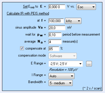
With this technique, the resistance of the solution can be determined by carrying out only one EIS measurement at high frequency, by default 100 kHz as shown in Figure 1 [4].

ZIR technique is available in EC-Lab^® software, whereas potentiostatic and galvanostatic techniques – respectively GZIR and PZIR – based on the same principle are available in EC-Lab^® Express software.

Figure 1: “Parameters Settings” window of ZIR experiment.

High frequency equivalent circuit of an electrochemical impedance

Equivalent circuit of an electro-chemical impedance

The equivalent circuit of an electrochemical impedance is given in Figure 2.

Figure 2: Equivalent circuit of an electrochemical impedance. C_dl is the double layer capacitance.

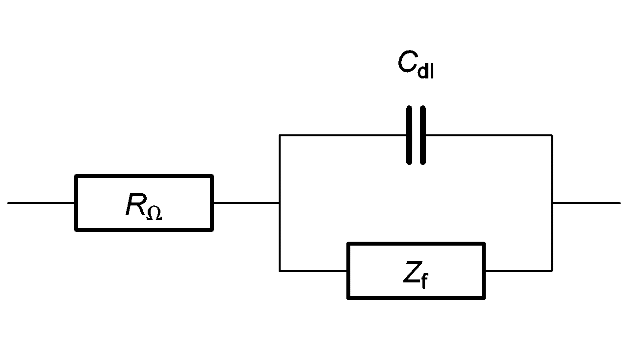
The equivalent circuit of the faradaic impedance Z_f depends on the electrochemical reaction involved.
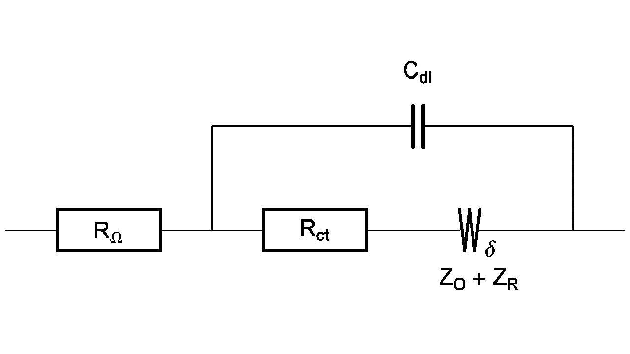
For example, the equivalent circuit of a redox reaction at a rotating disk electrode is shown in Figure 3 [5].

Figure 3: Equivalent circuit of a redox reaction at a rotating disk electrode.

High frequency equivalent circuit of an electrochemical faradaic impedance

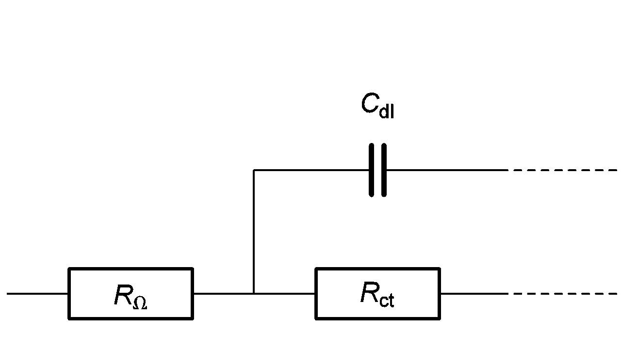
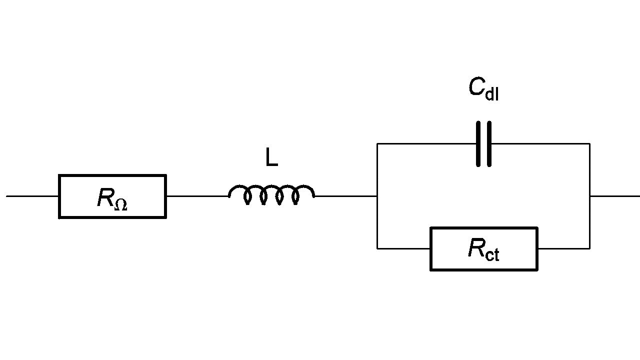
Let us consider the high frequency equivalent circuit of an electrochemical reaction shown in Figure 4. Z_f, given by:

$$Z_f=R_\Omega+\frac{R_{\mathrm{ct}}}{1+R_{\mathrm{ct}}\ C_{\mathrm{dl}}\ \mathrm{i}\ 2\pi\ f} \tag{2}$$

Figure 4: High frequency part of equivalent circuit shown in Figure 2.

The real part of Z_f is given by

$$\mathrm{Re}\ Z_f = R_\Omega+\frac{R_{\mathrm{ct}}}{1+4\pi^2\ f^2\ (R_{\mathrm{ct}}\ C_{\mathrm{dl}})^2} \tag{3}$$

with $\mathrm{lim}_{f\to \infty}\ \mathrm{Re}\ Z_f = R_\Omega$.

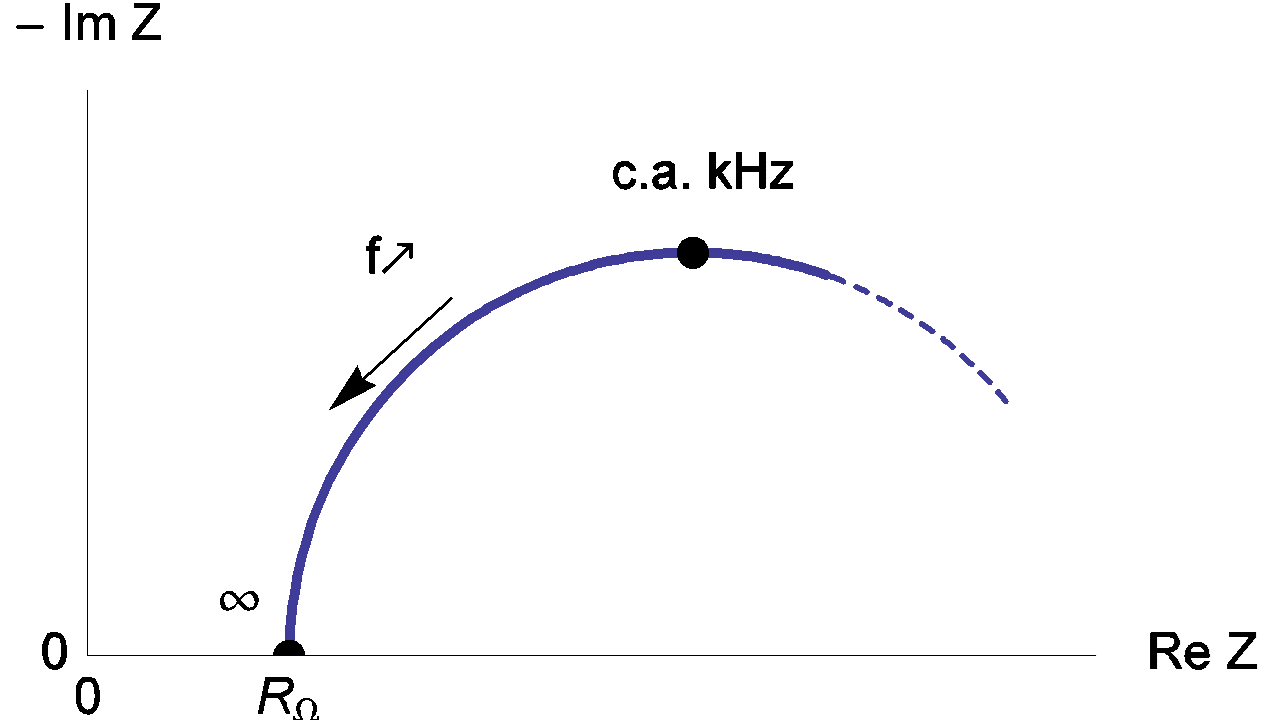
Therefore, the real part of the impedance Z_f tends towards R_Ω as frequency tends towards infinite as shown in Figure 5.

Figure 5: High frequency Nyquist diagram of the equivalent circuit of an electrochemical impedance.

R_Ω measurement in the simplest case

The real part of Z_f changes with frequency according to Eq. 3. Then the measurement relative error ε(f) can be defined as follows:

$$\varepsilon(f)=\frac{\mathrm{Re}\ Z_f\ -\ R_\Omega}{R_\Omega}=\left(\frac{R_{\mathrm{ct}}}{R_\Omega}\right) \frac{1}{1+4\pi^2 \tau^2 f^2} \tag{4}$$

Changes of the measurement relative error with various values of ratio R_ct / R_Ω are given in Figure 6.

Figure 6: Changes of the measurement relative error of R_Ω with frequency plotted for R_ct / R_Ω = 0.5, 1, 2, 5 and τ = R_ct C_dl = 10^-4 s. The line thickness increases with increasing R_ct / R_Ω ratio values.

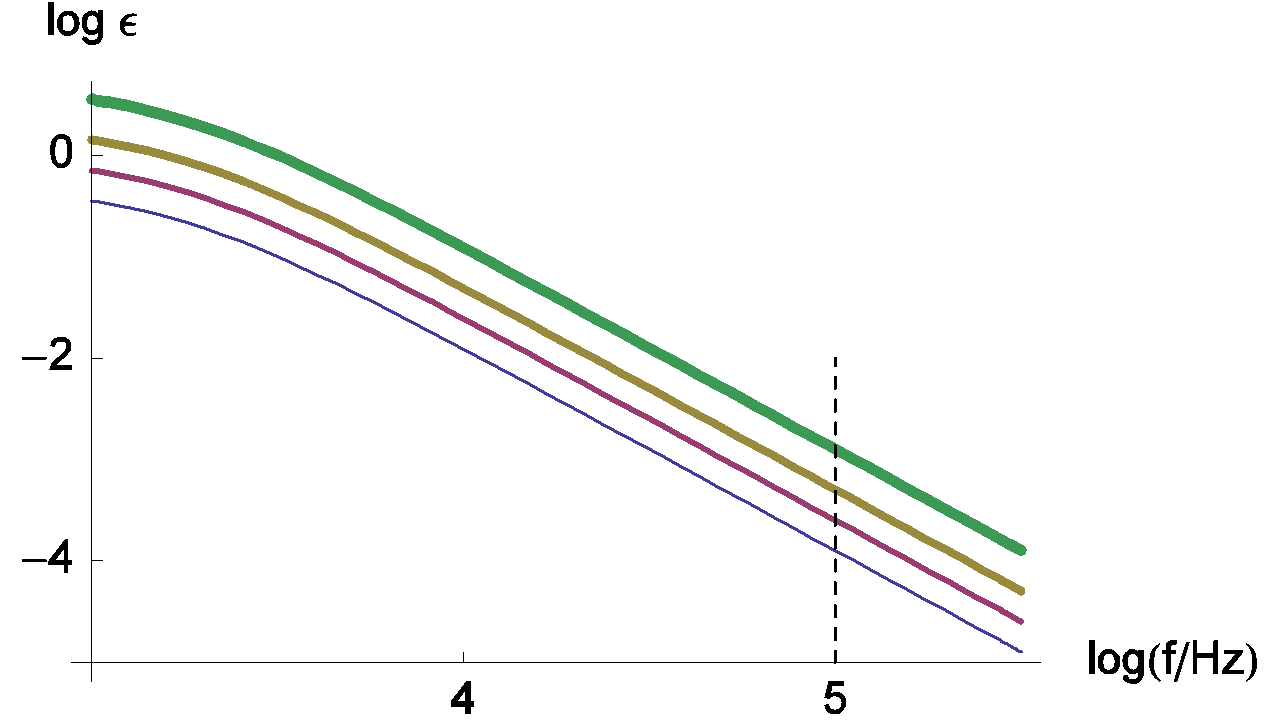
Generally, characteristic frequencies for the high frequency loop are in the kHz range. The frequency value used by default for the ZIR techniques is 100 kHz. In the previous figure, we can see that the relative error at 100 kHz is small and can be neglected; in this case the R_Ω measurement is correct.

R_Ω measurement with an inductance in series

Inductance in series

An inductive behavior can be observed at high frequencies for some electrochemical systems – batteries for example. Equivalent electrical circuits for this kind of system is given in Figure 7. The inductive part could be related to the connection or to the inductive behavior of the battery’s container.

Figure 7: High frequency equivalent circuit of a faradaic impedance considering an inductance in series.

Impedance of the circuit given Figure 7 can be written as follows:

$$Z_f=R_\Omega+L\ \mathrm{i}\ 2\pi\ f+\frac{R_{\mathrm{ct}}}{1+R_{\mathrm{ct}}\ C_{\mathrm{dl}}\ \mathrm{i}\ 2\pi\ f} \tag{5}$$

Depending on the L value, the shape of the impedance diagrams can change. Figure 8 gives an example of the various shapes of impedance diagrams that can be observed with an inductance in series. Curves displayed in Figure 8 can be reproduced with ZSim (EC-Lab^® software).

Figure 8: Nyquist impedance diagrams for the R+L+(R/C) circuit (Figure 7, (Eq. 3)). R_Ω = 0.2 Ω; R_ct = 1 Ω; C_dl = 10^-4 F, L = 10^-5; 2 x 10^-5, 5 x 10^-5, 10^-4 H. The line thickness increases with increasing L values.

Fortunately, the real part of the impedance is unchanged when compared to the previous example (R_Ω measurement in the simplest case) even with the addition of the inductance (L) (Eq. 5). Then the real part of Z_f for the R+L+(R/C) circuit is still given by Eq. 3. Moreover, the relative error curves on R are independent of the inductance (L) value. Then values displayed in Figure 9 are the same than those given in Figure 6.

Figure 9: Change of the measurement relative error of R_Ω with frequency. The parameters values are the same that the ones given in Figure 8.

(R/L) circuit in series

The high frequency behavior can be the one of an inductance in series but sometimes the behavior is the one of a (R/L) circuit in series (Fig. 10). Impedance of this circuit is given by

$$Z_f=R_\Omega+\frac{LR\ \mathrm{i}\ 2\pi\ f}{R+L\ \mathrm{i}\ 2\pi\ f}+\frac{R_{\mathrm{ct}}}{1+R_{\mathrm{ct}}\ C_{\mathrm{dl}}\ \mathrm{i}\ 2\pi\ f} \tag{6}$$

Real part of Z_f (Eq. 4) is given by

$$\mathrm{Re}\ Z_f = \frac{R_{\mathrm{ct}}}{1+4\pi^2\ f^2\ R_{\mathrm{ct}}^2\ C_{\mathrm{dl}}^2} + \frac{4\pi^2\ f^2\ L^2\ R}{4\pi^2\ f^2\ L^2\ R^2} + R_\Omega \tag{7}$$

This value depends of L and R.

Fig. 10: High frequency equivalent circuit of a faradaic impedance taking account of a (R/L) circuit in series.

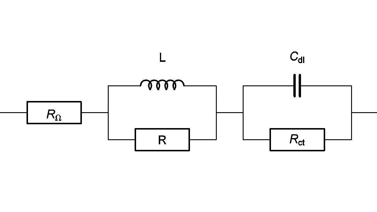
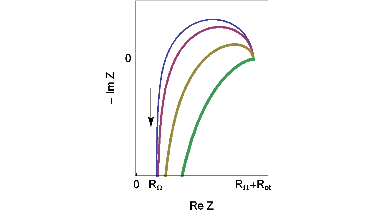
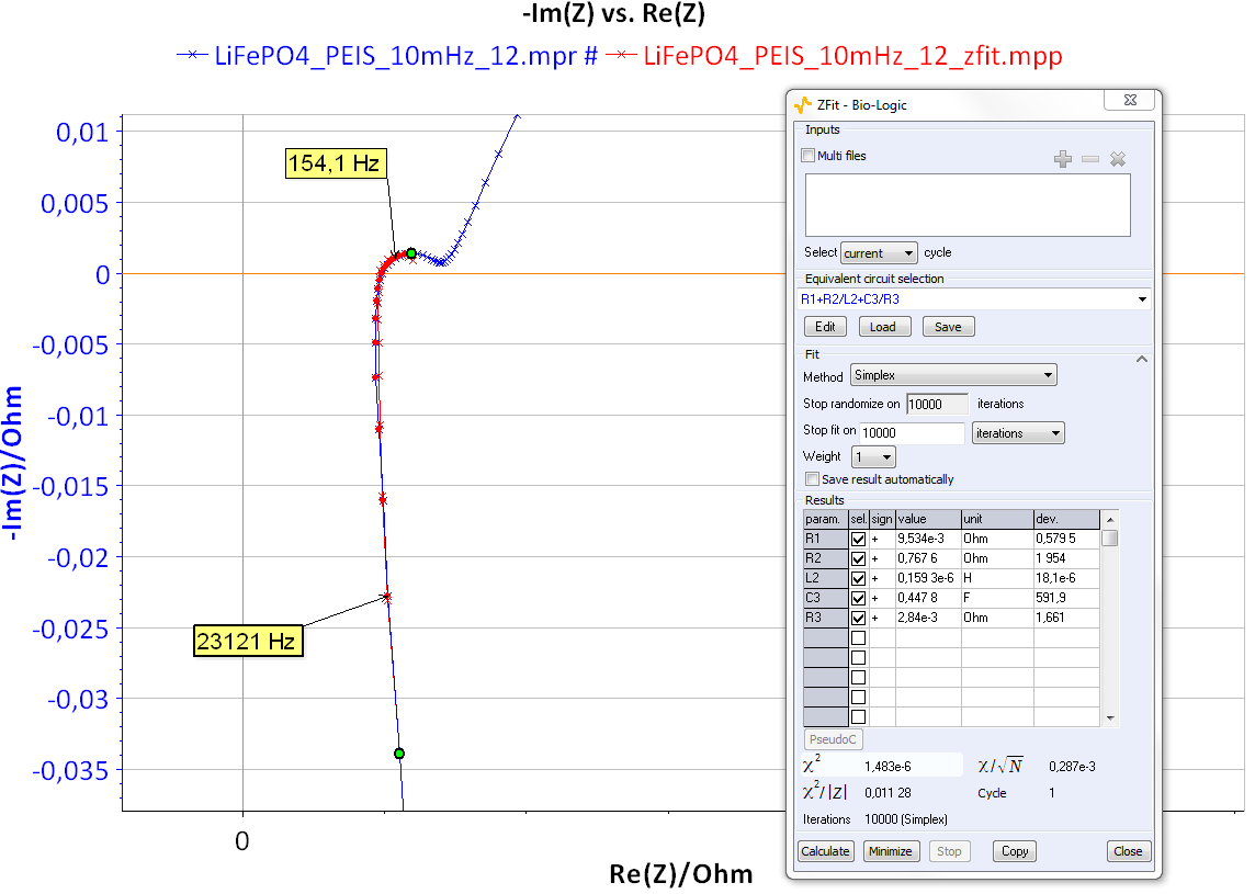
Figure 11 shows the Nyquist impedance diagrams obtained for the system R+(R/L)+(R/C). Note that different shapes for the Nyquist impedance diagrams can be obtained [5]. These kinds of Nyquist diagrams could be obtained with some batteries. An example of lead acid battery Nyquist diagrams can be found in the reference [6] or in Figure 12 for a LiFePO₄ battery.

Figure 11: Nyquist impedance diagrams for the R+(R/L)+(R/C) circuit (Fig. 11, (Eq. 4)). R_Ω = 0.2 Ω; R_ct = 0.5 Ω, R = 2 Ω; C_dl = 10^-4 F, L = 10^-7, 2 x 10^-6; 5 x 10^-6, 1.3 x 10^-5; 2.3 x 10^-5 (H). The line thickness increases with increasing L. Dots: minima of the real part of the impedance.

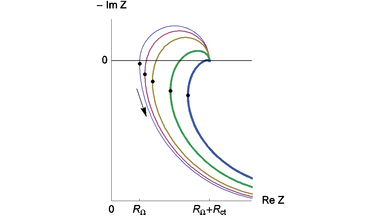
As previously, it is possible for the reader to obtain the curves displayed on Figure 11 with ZSim tool (EC-Lab^® software) or with the equivalent circuit library of the BioLogic website [5].

Figure 12: Nyquist diagram and ZFit analysis obtained on LiFePO₄ batteries.

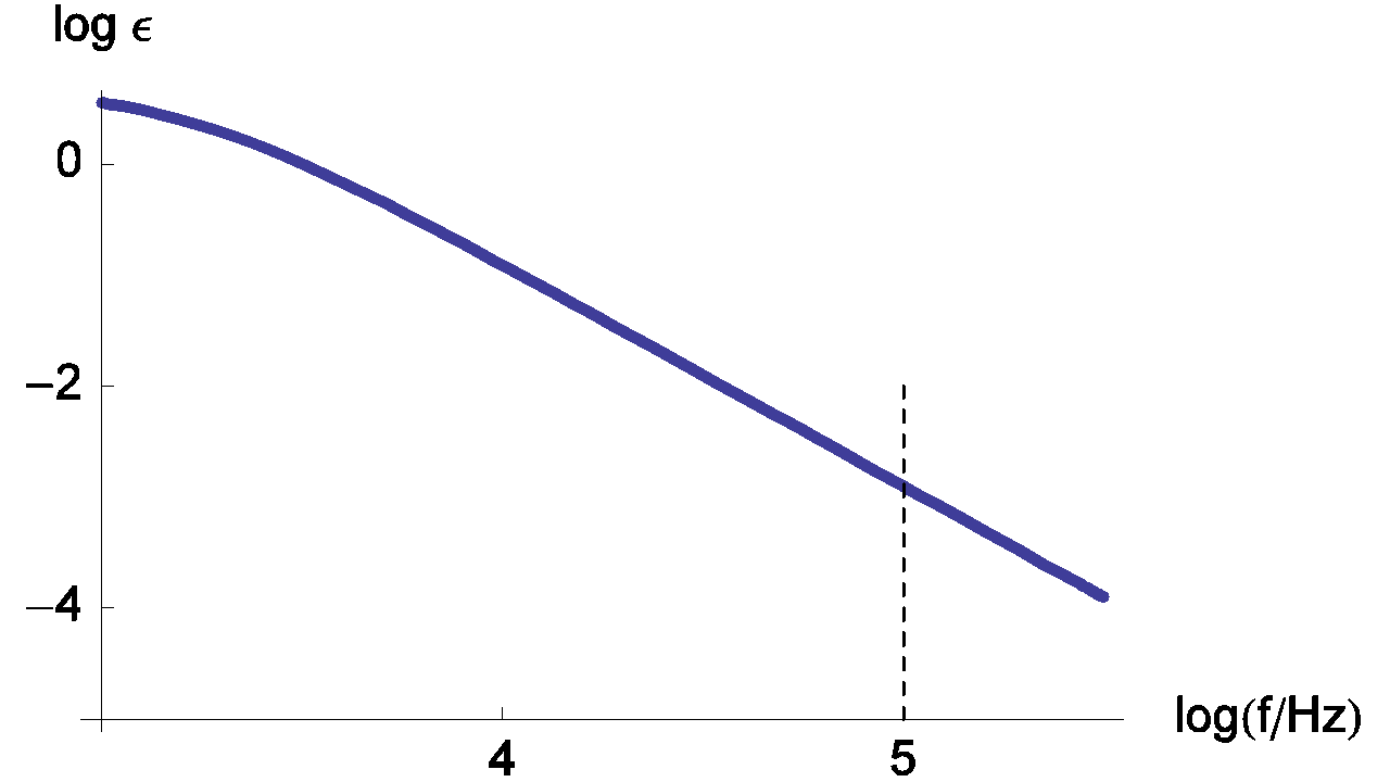
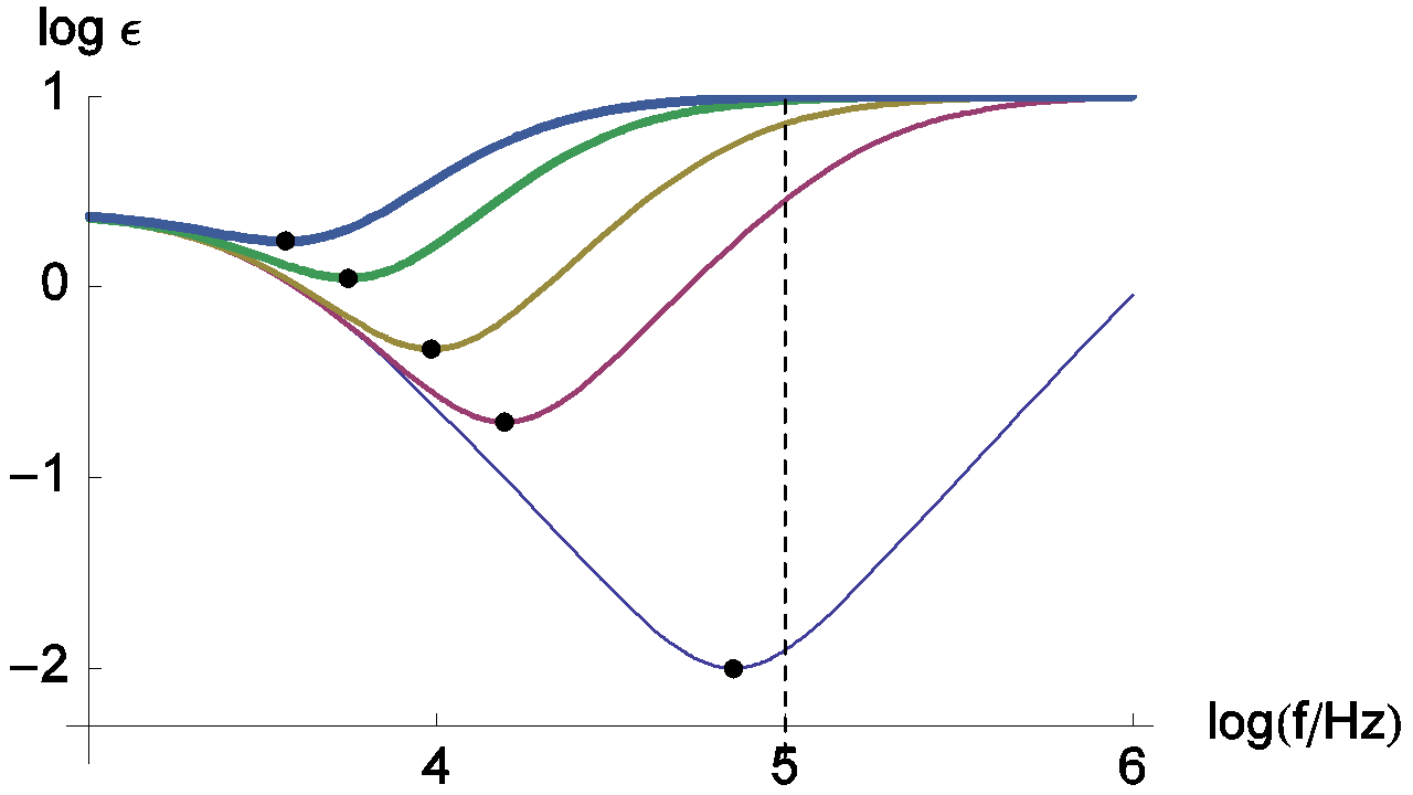
Changes of the relative error measurement on R_Ω are presented in Figure 13. This relative error doesn’t decrease monotonously when the frequency increases. In this case, the minimum of the relative error is obtained for the frequency corresponding to the impedance real part minimum, i.e. frequencies indicated by dots on the Figure 11.

Figure 13: Change of the relative error measurement of R_Ω with frequency. The parameters values are the same than those used in Figure 11. Dots: minima of the measurement relative error of R_Ω.