

Ohmic Drop Part II: Intro. to Ohmic Drop measurement techniques (Ohmic drop measurement) Battery – Application Note 28
Latest updated: May 5, 2023Abstract
The ohmic drop is RΩI where RΩ is defined as the solution resistance between the working electrode and the reference electrode plus any resistances in the working electrode itself, i.e. wires; I is the current flowing between the working and the counter electrode. Two methods are used in EC-lab® software to calculate this ohmic drop: electrochemical impedance (ZIR) and Current Interrupt (CI). A comparison of these methods is given in the note. It can be seen that the most accurate measurement of the ohmic drop is obtained by impedance.
Introduction
As explained in ref [1], ohmic drop can have a significant influence on the results of some experiments. It is therefore interesting to know how to determine the value of this resistance.
Various techniques can be used such as electrochemical impedance spectroscopy or current interrupt method. The aim of this application note is to compare these two methods.
EIS Measurement
In the first part of this note, Electrochemical Impedance Spectroscopy (EIS) measurement was carried out on circuit #1 of the TestBox-3. The behavior of this electrical circuit is linear as shown in ref [2]. This measurement was achieved with the PEIS technique at 0 V, with a frequency scan between 500 kHz and 1 Hz, a sinusoidal amplitude of 10 mV and the drift correction box ticked.
Nyquist diagram of the impedance for circuit #1 is shown in Figure 1.
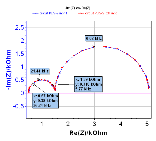
Figure 1: Nyquist diagram of the impedance of circuit #1-TestBox-3 (blue), resulting fit obtained with ZFit for the R1+C2/R2+C3/R3 equivalent circuit (red).
The electrical circuit #1 of the TestBox-3 is equivalent to the circuit given in Figure 2. In this circuit R1 mimics the ohmic drop resistance RΩ.
Thus an analysis with the EC-Lab® ZFit tool or EC-Lab® Express software allows the user to determine the value of each parameter. The results obtained are:
- R1 = RΩ = 499 Ω,
- C2 = 6.68·10-9 F,
- R2 = 1002 Ω,
- C3 = 2.30·10-6 F,
- R3 = 3569 Ω
and ZFit parameters are given in Figure 3.

Figure 2: Equivalent circuit of the electrical circuit #1 of the TestBox-3.

Figure 3: ZFit parameters.
The results obtained by EIS are in good agreement with the components’ values. The result of this measurement will help us to calculate the voltage step response to a current step for the circuit #1 of the TestBox-3.
Current Interrupt Method
The principle of the current interrupt method is an ohmic contribution appearance when an electrical contact is established. The reverse phenomenon happens: when the electrical contact is switched off, the ohmic contribution disappears instantaneously. Illustration describing the principle of this method is given in Figure 4 for a current step.


Figure 4: Current interrupt method principle with a current step.
Considering the previous EIS measurement and the principle of the current interrupt method, one knows that impedance of circuit #1 is given by:
$$Z(s)=R1+\frac{R1}{1+R2C2s}+\frac{R3}{1+R3C3s} \tag{1}$$
where s is the Laplace variable.
It is thus possible to calculate the circuit response using the inverse Laplace transform to a current step with amplitude ΔI:
$$E_{\mathrm{WE}}(t)= {L}^{-1}\left[\frac{\Delta I}{p}Z(p)\right] = \\ \Delta I\left(R1 + R2\left(1 – \mathrm{exp}\left(-\frac{t}{R2C2}\right)\right) + R3\left(1-\mathrm{exp}\left(-\frac{t}{R3C3}\right)\right)\right) \tag{2}$$
Two time constants τ2 = R2C2 = 6.7·10-6 s and τ3 = R3C3 = 8.2·10-3 s can be defined and be calculated. These two values are significantly different and only the main constant τ2 can be observed on the voltage step response with a linear time scale.
Considering the specifications of EC-Lab® and EC-Lab® Express software, respectively (200 µs and 20 µs acquisition time) and calculations carried out previously, it is possible to simulate the current interrupt method with a current step on the circuit #1 of the TestBox-3 and the measurement of the ohmic drop using the current interrupt method (Figure 5).

Figure 5: Simulation of current interrupt method (0.1 mA) on the circuit #1 of the TestBox-3 considering EC-Lab® and EC-Lab® Express specifications. RΩI is the true ohmic drop. R’I and R’’I represent the ohmic drop measured respectively with EC-Lab® and EC Lab® Express software.
With EC-Lab® , software measurement is carried out every 200 µs. Then the first measured potential is 0.15 V. Considering Ohm’s law and the applied current (0.1 mA), it is then possible to calculate R’ I = 0.150 V, then R’ = 1.5 kΩ.
With EC-Lab® Express software, the measurement takes place every 20 µs. In this case the first point is obtained at 0.074 V. It is then possible to calculate R” I = 0.074 V, then R” = 1.1 kΩ.
The two values obtained are not in agreement with the theoretical value of the ohmic drop resistance RΩ, which is 499 Ω. Indeed, depending on the software and consequently the minimum acquisition time period, the experimental value obtained is close to R1+R2 for EC-Lab® software and between the value of R1 and the value of R1+R2 for EC-Lab® Express software.
Battery Analysis
A 18650 lithium-ion battery, with a capacity of 1.2 Ah, was studied. The positive electrode is composed of LiFePO4, the negative one of graphite carbon and the electrolyte is a lithium salt.
EIS Measurements
Before the impedance measurement, the system was maintained for 30 s at 3.10 V, and the frequency scan was carried out between 50 kHz and 10 mHz, with an amplitude equal to 10 mV, pw = 1 before each frequency measurement and the drift correction method used. The Nyquist diagram is given in Figure 6.
ZFit analysis was obtained in the [0.022 – 7.27] kHz frequency range (cf. Figure 6). The equivalent circuit in the high frequencies domain is close to L1+R1+Q2/R2. The value of R1 determined with the ZFit analysis tool is ~9.13·10-3 Ω. A summary of the obtained values is given Figure 7.
![Nyquist diagram of LiFePO4 battery (blue) and resulting fit (red) obtained with ZFit for the L1+R1+Q2/R2 equivalent circuit in the [0.022 7.27] kHz frequency range.](https://biologic.net/wp-content/uploads/2019/08/an28f6a.png)
![Nyquist diagram of LiFePO4 battery (blue) and resulting fit (red) obtained with ZFit for the L1+R1+Q2/R2 equivalent circuit in the [0.022 7.27] kHz frequency range.](https://biologic.net/wp-content/uploads/2019/08/an28f6b.png)
Figure 6: Nyquist diagram of LiFePO4 battery (blue) and resulting fit (red) obtained with ZFit for the L1+R1+Q2/R2 equivalent circuit in the [0.022 – 7.27] kHz frequency range.
Note that it can sometimes be useful to estimate the value of the battery resistance by direct reading on the EIS diagram when Im(Z) = 0 Ω. When executing this approximation, an error can be encountered. Indeed in this example a direct reading gives a value of ~ 9.8·10-3 Ω, whereas the ZFit calculated value is ~ 9.13·10-3 Ω, this means a difference of ~ 10% between these two values.
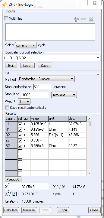
Figure 7: ZFit analysis window.
Current Interrupt Method
As previously stated for the electrical circuit let us simulate the step response of the L1+R1+Q2/R2 circuit obtained with EIS measurements. Due to the real value of a2 it is not possible to determine in a closed form the inverse Laplace transform of
$$E_{WE}(t)=L^{-1}\left[\frac{\Delta I}{p}Z(p)\right] \tag{3}$$
for the Lithium-ion battery. Fortunately, efficient algorithms are available for numerical inversion of Laplace Transform (NILT) [3,4].
It is then possible to simulate a current step of 400 mA applied on the battery. This simulation was achieved with the parameters related to EC-Lab® and EC-Lab® Express software. The result of the simulation with the two software is shown in Figure 8.
Considering this figure the first recorded point with EC-Lab® software is obtained for a potential of ~ 3.104 V. Indeed following Ohm’s law, we have the relationship R’ ΔI = ΔE, where ΔE is the difference between the initial potential of the battery (~ 3.098 V) and the first recorded potential (~ 3.104 V), i.e. ΔE ~ 6·10-3 V. Then R’ with EC-Lab® software is equal to 0.014 Ω.
The same calculation can be achieved with EC Lab® Express software considering the potential of the first recorded point (~ 3.104 V). Considering Ohm’s law and ΔE, which is the difference between initial potential of the battery (~ 3.099 V) and first recorded potential (~ 3.104 V), i.e. ΔE = 5·10-3 V, R” is equal to 0.012 Ω.

Figure 8: Simulation of perfect current step (400 mA) on lithium-ion battery considering EC Lab® specifications. RΩI is the real ohmic drop. R’I and R”I represent the ohmic drop obtained respectively with EC-Lab® and EC Lab® Express software.
Results obtained with EIS measurements and the current interrupt method are close to each other for this system with slow kinetics. Moreover, these results are close to the theoretical value of the ohmic drop resistance which was not the case for the measurements obtained on the electrical circuit.
Conclusion
This note demonstrates the limitations imposed by the current interrupt method. Indeed depending on the kinetics of the system, this method is more or less accurate. Note that the right value of ohmic drop resistance is never obtained. Impedance measurement is a well-adapted tool and gives the right value of the ohmic drop whatever the kinetics of the system.
Note that a special tool was developed in the EC-Lab® and EC-Lab® Express software which offers the possibility to measure by EIS and compensate for the ohmic drop. This tool allows the user to obtain an immediate value of the ohmic drop without the need to know the electrical equivalent circuit. Note that, by default, this measurement is obtained for 100 kHz, but the user can change this value according to the system being studied.
For example, considering the previous studied systems, the determination of the ohmic drop was achieved with with:
- The PZIR technique of EC-Lab® Express software. Obtained results are 502.6 Ω at 500 kHz for the circuit and 9.77·10-3 Ω at 800 Hz for the lithium-ion battery
- The ZIR technique of EC-Lab® software. Obtained results are 501.3 Ω at 500 kHz for the circuit and 9.76·10-3 Ω at 800 Hz for the lithium-ion battery.
Nevertheless, one can ask why is there such a sampling difference between current interrupt and EIS methods. This is because in EIS we use the undersampling or Super-Nyquist sampling method. This is a well-known concept, which allows us to measure single tone frequencies over the sampling rate of the instrument.

Figure 9: Undersampling scheme.
Data files can be found in:
C:\Users\xxx\Documents\EC-Lab\Data\Samples\EIS\ LiFePO4_PEIS_10mHz_12 and
Application Note 09\PEIS_circuit1
References
- Application Note #27 “Ohmic Drop, Part I: Effect on measurements”
- Application Note #9 “Linear vs. non-linear systems in impedance measurements”
- C. Montella, R. Michel, J.-P. Diard, J. Electroanal. Chem., 608 (2007) 37.
- C. Montella, J.-P. Diard, J. Electroanal. Chem., 623 (2008) 29.
Revised in 08/2019


