Ohmic Drop Part I: Effect on measurements (Ohmic drop effect on measurements) Battery & Corrosion – Application Note 27

Introduction

The ohmic drop (IR drop) describes the over-potential due to the electron flow through a material. In electrochemistry, it often refers to the potential induced by the resistance of the electrolyte or any other interface (Fig. 1) such as surface films or connectors [1].
For a voltammetry on a given system, the applied potential, in presence of an ohmic drop, should abide by the following equation:

$$E(t)=E_i+v_bt-R_\Omega I(t) \tag{1}$$
where E_i is the polarization potential, ν_b is the scan rate and t is the time.

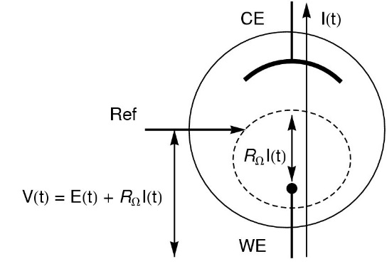
Figure 1: Schematic of ohmic drop in the standard three-electrode set-up (V: potential applied by the potentiostat; E: potential at the electrode and RΩI: ohmic drop).

As we will show in this note, ohmic drop can have an influence on the shape of the measured curves and also be a source of error during the analysis of results. In this context, the effect of the IR drop on several electrochemical techniques are highlighted.

N.B.: All settings and raw data files presented hereafter are available in the Data Sample folder of EC-Lab^® Software with the following name: techniquesXOhm_ODI.mpr.

Steady-State Conditions

The ohmic drop has an effect on the shape of voltammetry measurements.
N.B.: It is important to note that the ohmic drop effect is a critical parameter for ultra-fast scan rate investigation [2].

Voltammetry

In this context, steady-state voltammetry is performed according to settings described in Fig. 2.

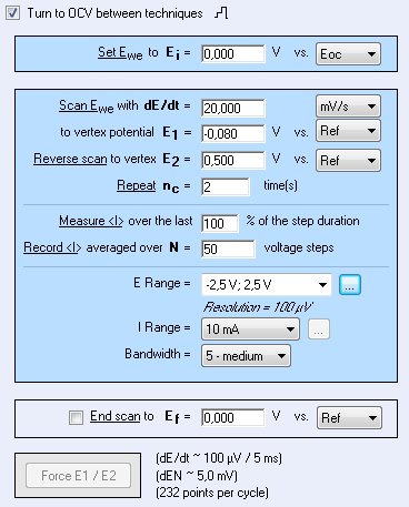
Figure 2: Voltammetry settings window.

Investigations are carried out with a solution of [Fe(CN)₆]^3- (0.6 mM) with KCl as supporting salt (0.5 M). A three-electrode set-up is used with the following configuration:

• Platinum electrode (surface electrode A = 3.14 mm^-2) as working electrode (WE),
• Standard Calomel Electrode (SCE) as reference electrode,
• Platinum wire as counter electrode.

Scan rate and rotating rate are of 20 mV·s^-1 and 2,000 rpm, respectively.
The resulting curves are presented in Fig. 3.

Figure 3: Steady-state curves of [(Fe(CN)₆]^3- (0.6 mM) + KCl (0.1 M). No resistance (red) and resistance of 100 Ω (blue) added in series with the WE.

The effect of the ohmic drop appears clearly in Fig. 3 and the difference of potential between both curves for each current value is equal to R_ΩI. For example, at -500 µA, potentials are 150 and 98 mV without and with additional resistance, respectively. This yields to a resistance of about 100 Ω.

Tafel Plot

The user must be careful when trying to determine the corrosion current, for example, with Tafel plot analysis from the LP curves of circuit #2 of TestBox-3 according to the settings presented in Fig. 4 [3].

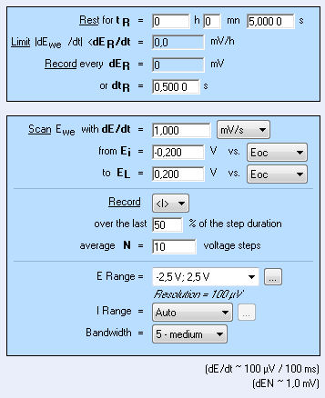
Figure 4: LP Settings window.

As shown in Fig. 5 the ohmic drop has an influence on the curves plotted in log |I| vs. E_we.
In the cathodic and the anodic areas (red arrow in Fig. 5 ), the curve with the additional resistance of 1 kΩ doesn’t exhibit linear behavior, but that of a curved one due to the ohmic drop. That is why the Tafel Fit of each curve gives different results. In this case, the current corrosion of the curve obtained without additional resistance (I_corr = 23 nA) is twice those obtained with the additional resistance (I_corr = 44 nA).

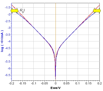
Figure 5: Steady-state curves of circuit #2 of TestBox-3. No resistance (red) and additional resistance of 1 kΩ (blue) in series with the WE.

Another Example

The addition of a resistor can also induce some tricky behavior.
For example, the steady-state curve of circuit #3 with the settings of Fig. 6 results in a typical peak for a Z-shaped curve.
But if a resistance (for instance: 1 kΩ) is added in series with the WE in order to simulate the ohmic drop, the shape of the resulting curve is totally modified i.e. the shift of the potential maximum and the appearance of a hysteresis phenomenon between forward and reverse scan (Fig. 7). This phenomenon is due to the specific behavior of this circuitry.
From the shift potential, it is possible to calculate the resistance of the ohmic drop. For example, in this experiment the potential shift is 1.7 V and the current at the maximum is 1.7 mA which corresponds to a resistance of 1 kΩ.

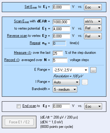
Figure 6: CV setting window.

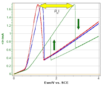
Figure 7: Steady-state curves of circuit #3 of TestBox-3. No resistance (red), resistance of 100 Ω (blue) and 1 kΩ (green) added in series with the WE.

Impedance Measurements

The ohmic drop is very easy to determine from impedance measurements in the Nyquist plot. It is often associated with the ohmic resistance RΩ which can be identified looking at the real part of impedance for high frequencies [4]. Indeed, the ohmic drop can be modeled in an electrical circuit by adding a resistance in series between the working electrode and the reference electrode [1].
Nyquist plots were obtained by performing Potentio Electrochemical Impedance Spectroscopy (PEIS) investigations on circuit #3 of TestBox-3 based on the settings of Fig. 8. A resistance of 100 Ω or 1 kΩ is added to the circuit to simulate the ohmic drop. By looking at the diagram (Fig. 9), the ohmic drop effect is obvious. Indeed, the shift at high frequency is due to the presence of the additional resistances.

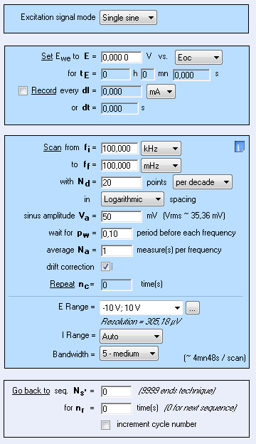
Figure 8: PEIS Settings.

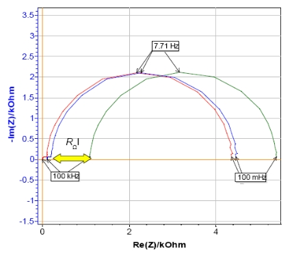
Figure 9: Nyquist plot of circuit #3 of TestBox-3 in the. No resistance (red), resistance of 100 Ω (blue) and 1 kΩ (green) added in series with the WE.

Non Steady-State Condition

Non-stationary curves were also plotted for the system described in the “voltammetry” section based on the settings shown in Fig. 10. Results (Fig. 11) show an influence of the ohmic drop on the potential peak AND also on the current.

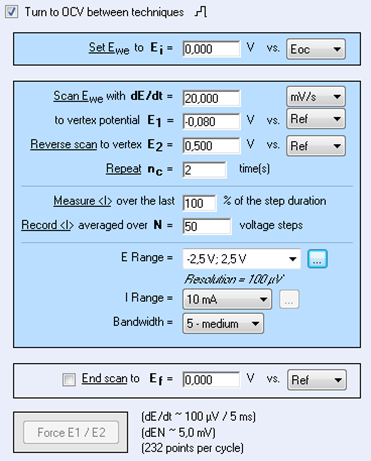
Figure 10: CV setting window.

Figure 11: CV curves of [(Fe(CN)₆]^3- (0.6 mM) + KCl (0.1 M). No resistance (red) and resistance of 100 Ω (blue) added in series with the WE.

Indeed, on one hand, potential peaks are shifted towards cathodic values for the reduction peak and towards anodic values for the oxidation peak. On the other hand, maximum current values are under-estimated. These two changes could mislead the user to think the electrochemical system is slower than it actually is.

References

- J.P. Diard, B. Le Gorrec, C. Montella, Cinétique électrochimique, Hermann, Paris (1996) 17.
- C. Amatore, E. Maisonhaute, G. Simonneau, Electrochem. Comm., 2 (2000) 81.
- D. Landolt, Traité des Matériaux, 12, Corrosion et Chimie de Surfaces des Métaux, Presses Polytechniques et Universitaires Romandes, Lausanne (2003) 184.
- Application note 23, “EIS measurements on Li-ion batteries – EC-Lab software parameters adjustment.”
- Application note 28, “Ohmic Drop. II – Introduction to Ohmic Drop measurement techniques.”
Revised in 08/2019