EIS measurements on Li-ion batteries EC-Lab^® software parameters adjustment (EIS optimizations) Battery – Application Note 23

Introduction

To obtain significant EIS plots, without experiencing noise or other issues, experimental parameters should be chosen carefully. Users should also pay attention to the definition of each parameter and test the effects of each one on the results.
Furthermore, all electrochemistry software is designed differently, and users must adapt parameters according to their own particular software interface.
The aim of this note is to help the user obtain good experimental results with EC-Lab^® software. To this end, a detailed description of some key points (connections, cable length, experimental parameters etc.) is explained below.

Experimental Part

In the following application note, experiments were carried out on a Li-ion battery with a nominal capacity of 10 Ah. Experiments were executed at the E_oc potential, i.e. 3.3 V.

Note that experiments were obtained with EC-Lab^® software in potentiostatic mode.

Connection

Two kinds of two electrodes connections can be considered:

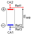
1) The “two-point” connection with CA2+Ref1 together on the positive electrode and CA1+Ref2+Ref3 together on the negative electrode:

2) The “five-point” connection by separating each cable on each electrode, i.e. CA2 and Ref1 on the positive electrode and CA1, Ref2, and Ref3 on the negative electrode:

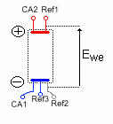
This connection is also recommended for ac-curate potential measurements.
As shown in Figure 1, we can notice a shift of + 2.5 mΩ between the EIS diagram obtained with the banana plugs connected together (1) comparing with the banana plugs connected separately (2).

Figure 1: Comparison of EIS diagrams obtained with two-point connection (green line and markers) and five-point connection (red line and markers).

This example shows that for systems with a small resistance, the connection is very important and can significantly influence results. This is why it is necessary to minimize the value of stray capacitance, stray inductance or resistance [1] generated by the connection. Each connection lead should be separated and connected as close as possible to the electrochemical system to reduce the intrinsic influence of the connection.

Cable Length

Lengthened cables are sometimes deemed necessary for certain configurations. However, this should be avoided wherever possible, as extended cables can impact negatively on result quality.
We used a standard cable (red EIS curve) and a cable of 10 m length (blue EIS curve) for these experiments. Note, that to avoid oscillations of the potentiostat, resistors were added to the reference plugs on the 10 m cable.
As shown in Figure 2, a slight difference can be noticed between the EIS curves obtained with the standard and long cables. Depending on the system studied, EIS measurements with long cables should be analyzed with caution.

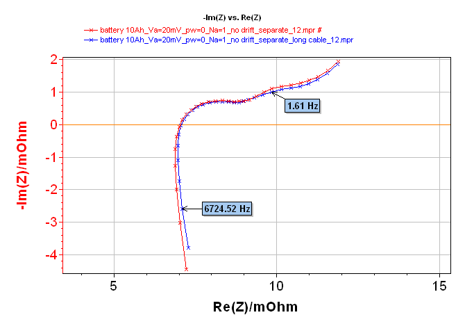
Figure 2: Comparison of EIS curves obtained with a standard cable (red curve and markers) and with a 10 m cable (blue curve and markers).

Experimental Parameters

PEIS technique experiments (Figure 3).

Excitation amplitude
The first parameter to determine is the value of the potential excitation V_a. Note that before the 9.56 EC-Lab^® version, excitation amplitude was defined as V_a (sinus amplitude). Equivalence between V_a, V_pp (peak to peak amplitude) and VRMS is defined by the relationship:

$$V_a=\frac{1}{2}V_{pp}=\sqrt2V_{RMS} \tag{1}$$

This parameter value has to be chosen considering the current amplitude |I| and the potential amplitude |E| values. The |I| and |E| are the amplitude applied around the DC level of current or around the DC level of potential. It is the AC amplitude. In EC-Lab^® software, DC levels of current or of potential are called I and E. The V_a value has to be determined in such a way to ensure the system is linear in order to obtain significant EIS results [2].

Figure 3: “Parameters Settings” window of PEIS experiment.

Firstly, a V_a value of 0.5 mV was chosen. The obtained EIS diagram is given in Figure 4.

Figure 4: EIS diagram obtained with the following experimental conditions: Va = 0.5 mV, pw = 0, Na = 1 and no drift correction.

Considering the poor quality of this EIS diagram, we should analyze current and potential amplitude values, which are significant for EIS measurements (Figure 5 & Figure 6).
Indeed, the value, which is the open circuit potential of the battery, is not significant for the EIS measurement, but as expected, this value is maintained during the measurement.
The value of |E_we|, which is the modulus of the applied potential modulation is very small, only 0.5 mV (Figure 5). Considering the specifications of the instrument in impedance, signals smaller than 1 mV present the same level as the noise. At this point, in this measurement, the value of potential amplitude (|E_we|) is included in the measurement noise that explains the poor quality of the EIS diagram.

Figure 5: Change of potential amplitude IEweI with frequency.

The value of |I| is small but in good agreement with the accuracy of the instrument (Figure 6).

Figure 6: Change of current amplitude III with frequency.

In this experiment, the critical parameter is the amplitude of potential. Note however, that the current and/or potential can be critical parameters depending on the studied system.
To improve the EIS diagram, the V_a value has to be changed. Considering the previous results, it seems that an increase of the V_a value could help to obtain a good quality EIS diagram.
Figure 7 gives the EIS diagram obtained with 10 mV as V_a value.

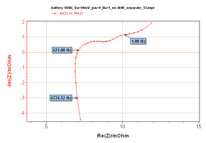
Figure 7: EIS diagram obtained with the following experimental conditions: Va = 10 mV, pw = 0, Na = 1 and no drift correction.

This time, the value of the potential amplitude (|E_we|) is significant and in agreement with the accuracy of the instrument.
The influence of the increase of the V_a value can clearly be seen on the comparison between EIS diagrams obtained with V_a = 0.5 mV and with V_a = 10 mV as shown in Figure 9.

Figure 8: Top: Change of potential amplitude |E_we| with frequency. Bottom: Change of current amplitude |I| with frequency.

Figure 9: Comparison of EIS diagrams obtained with a potential excitation Va of 0.5 mV (purple curve) and of 10 mV (red curve).

The p_w value
The p_w box offers the user the ability to add a delay before the measurement at each frequency. This delay is defined as a fraction of the period. In other words, this delay offers users the ability to let the system come out of a transient period resulting from the frequency transition and back to a steady-state sinusoidal behavior. This parameter is important especially for systems with a large time constant.
The aim of this part of the measurement is to show the effect of p_w value on the EIS diagram in comparison to a well-defined diagram (for V_a = 10 mV). Figure 10 shows a comparison between two EIS diagrams obtained with two values of p_w (0 and 1) and V_a = 0.5 mV and one diagram obtained with V_a = 10 mV and p_w = 0.

Figure 10: Comparison of EIS diagrams obtained with V_a = 0.5 mV, N_a = 1 with no drift correction and a value of pw equal to 0 (purple curve) or 1 (blue curve) with EIS diagram obtained with V_a = 10 mV (red curve).

Firstly, we can see that the diagram obtained with the value of p_w = 1 is less noisy than the one obtained with p_w = 0. Moreover, this diagram obtained with pw = 1 is almost superimposed with the “correct” EIS diagram obtained with V_a = 10 mV.
This result means that it is possible to compensate slightly for a noisy shape of an EIS diagram just by increasing the p_w value and without disturbing the cell much. This result is in agreement with a high time constant of the system. Of course, this increases the experiment time. For example in this experiment for a value of p_w of 0, a time of 6 s is needed for one scan, whereas when the value of p_w is 1 a time of 13 s is needed for one scan.

The N_a value
N_a is the number of repetitions of measurements at each frequency, and then an average is carried out for each frequency. This means that the noise is reduced following the mathematical law .
In the following section, two values of N_a were tested 1 and 36, the other parameters are equal: V_a = 0.5 mV, p_w = 0, no drift correction, separate connection. The full frequency sweep is repeated 15 times to show the data point dispersion.
Figure 11 shows the results obtained with N_a = 1. It is possible to see that for each frequency the recorded points are not superimposed. It is clearly visible on the enlargement.
Figure 12 shows the experiment done with N_a = 36. Obviously, for each frequency, recorded points are superimposed, meaning that the coordinates of each recorded point are not more affected by the surrounding noise.

Figure 11: Repetition of EIS diagrams obtained with the following experimental conditions: V_a = 0.5 mV, p_w = 0, N_a = 1 and no drift correction. Top: complete diagram, bottom: enlargement.

Drift correction
The drift correction tool is especially dedicated to systems with very long relaxation times. Indeed, the unsteadiness of systems can induce a slight deviation on the obtained impedance graphs compared with a theoretical one. This tool is explained extensively in reference [3].