

Drift correction in electrochemical impedance measurements (EIS non stationarity) Battery – Application Note 17
Latest updated: March 12, 2025Abstract
An electrochemical impedance measurement is valid if the system is linear, time-invariant and causal. The time needed by a system to reach its stead-state and consequently the electrochemical impedance measurement can take can be very long. To avoid waiting for the steady-state of the system, the “Drift correction” feature can be used. This option compensates the effect of the transient state of the system on its response to the sinusoidal modulation used in impedance measurements. Generally the error caused is seen at lower frequency. Some examples of used are impedance measurements on batteries under charge or discharge, impedance measurements at various DC bias of a corroding system. “Drift correction” is a patented feature.
Introduction
Several conditions are required to measure the electrochemical impedance of a system. Its behaviour must be linear, invariant vs. time, and the system should be in a steady-state. Indeed, if the steady-state is not reached by the system, the electrochemical impedance signal used to calculate the Fourier Transform is not periodic. Moreover, the presence of a transient period due to the excitation step implies in the result spectrum,, a contribution to the response of the imposed sinusoid (Figure 1).

Figure 1: Example of a current response to an excitation by a sum of a potential step (amplitude: ΔE) and a series of sinusoids (amplitude: δE). Left: sinusoids series starting when the steady state is reached. Right: sinusoid series starting at the beginning of the potential step.
This application note deals with a drift correction method in impedance measurements when it is carried out in drift conditions just toward the steady-state. Fourier Transform of the input and output signals are used to implement the drift correction. In the first part of the note, a measurement error example is given for an electrical circuit, and the second part gives the comparison of measurements carried out for a lithium-ion battery with and without drift correction.
Experimental Part
All the impedance measurements shown in this application note were obtained with the EIS technique of EC-Labâ Express software (cf. Figure 2), generally with a potential step amplitude of ΔE = 10 mV. Different cycles were carried out for each measurement (measurements were executed successively).
Note: the drift correction tool is also available in EC-Lab® software.

Figure 2: PEIS technique diagram in the EC-Lab® Express software with the drift correction box ticked.
Impedance Measurement in Drift Conditions Toward A Steady State
Electrical Test Circuit
Figure 3 shows an electrical circuit made of 3 capacitors and 2 resistors.

Figure 3: Electrical test circuit.
Impedance of this linear circuit is well known when a potential step with a ΔE amplitude is applied [1]. Nevertheless, studying this circuit can give an example of the drift correction method. Figure 4 shows the measured transient current corresponding to the electrical circuit response to a potential step. Let us consider that the current value is close to zero after ~ 2 min. Thus, to measure the impedance of this steady state circuit, it is necessary to wait 2 min before starting the measurement.

Figure 4: Current response of the electrical circuit (Figure 3) to a potential step.
Three impedance Nyquist graphs – corresponding to cycles – of the electrical circuit (Figure 3) measured successively without waiting for the steady state are given in Figure 5.
A difference in the middle frequency range for the second arc of circle (intermediate frequencies) is visible. The second and third cycles are close to each other and correspond to the graph obtained at the open circuit potential. The measurement duration is around 8 min, and the second and third cycles are plotted in steady-state conditions. This is not the case for the first graph.
Reaching the steady state can take a long time, which is not always convenient for doing series measurements. This can therefore be a useful time-saver.

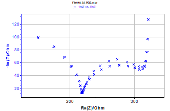
Figure 5: Three impedance Nyquist graphs of the electrical circuit (Figure 3) measured successively from the potential step application. Enlargement of the low frequencies area is also given. (fmin = 20 mHz, fmax = 100 kHz (51 measured points), ΔE = 50 mV, ΔE = 10 mV).
Principle of the Drift Correction Method Toward A Steady State
Several methods are available to define the drift correction [2,3,4-7]. The method given in this note is based on the Fourier transform impedance measurement. This method consists of the calculation of discrete potential and current Fourier transforms. Correction is carried out by compensation using the $f_{m-1}$ and $f_{m+1}$ adjacent frequencies of $f_m$ in the Fourier spectrum, with the following equations:
$$\mathrm{Re}I_{corr} = \mathrm{Re}I(f_m)\ – \frac{\mathrm{Re}I(f_{m+1})+\mathrm{Re}I(f_{m-1})}{2} \tag{1}$$
$$\mathrm{Im}I_{corr} = \mathrm{Im}I(f_m)\ – \frac{\mathrm{Im}I(f_{m+1})+\mathrm{Im}I(f_{m-1})}{2} \tag{2}$$
The principle of this correction is shown in Figure 6. Without drift, $\mathrm{Re}I(f_{m+1})$, $\mathrm{Re}I(f_{m-1})$, $\mathrm{Im}I(f_{m+1})$ and $\mathrm{Im}I(f_{m-1})$ are null and drift correction does not modify the measurement.

Figure 6: Principle of drift correction method for an imposed potential. (Real part of the Fourier spectrum).
An example of the drift correction is given in Figure 7 for the Figure 3 circuit. These measurements were obtained successively from the potential step application. The three graphs are close and in agreement with results obtained in open circuit.
The drift correction method used towards a steady-state reduces the impedance experiment’s measurement time for an electrical circuit submitted to a potential step.


Figure 7: Three impedance Nyquist graphs with drift correction of Figure 3 circuit measured successively from the potential step imposition.
Study of A Lithium-Ion Battery
This drift correction method was applied on a 1.35 Ah Sony Energytec Li-Ion battery. Characterization of lithium-ion batteries is often achieved with a series of partial charges/discharges with current or potential limitations, and an open circuit period. The duration of this relaxation period could be very long due to the slow diffusion coefficient of the intercalated species into the host material (~ 10-12 mol·cm-2). Indeed, Figure 8 shows the current response of this battery to a potential step and the time (~ 1 h 00) required to reach equilibrium state.

Figure 8: Lithium-ion battery current response to a potential step (EOC = 3.09 V).
Measurement without Drift Correction
The two impedance graphs of the lithium-ion battery measured in potentiodynamic mode are given in Figure 9. These graphs were recorded from the potential step application. Measurement total time is around 1 h 20 min. These two graphs – corresponding to different cycle – present significant differences mainly in the low frequencies range (Figure 9).


Figure 9: Lithium-ion battery impedance Nyquist graphs successively measured and low frequency enlargement. (fmin = 5 mHz, fmax = 10 kHz, 51 measurement points, δE = 3 mV, EOCV = 3.09 V).
Measurement with Drift Correction
Results obtained for lithium-ion battery impedance measurement with drift correction are given in Figure 10. These two impedance graphs are very close, as shown in the low frequency enlargement. The drift correction allows the user to save time for battery impedance measurement.
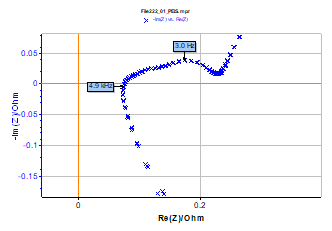

Figure 10: Lithium-ion battery impedance Nyquist graphs successively measured and low frequency enlargement; measurements done with drift correction. Same conditions as those of Figure 9.
Conclusion
The drift correction method proposed in this note is very easy to use with only the measurements of two sinusoid periods. This method is a good way to perform impedance measurements on systems with very long relaxation times. This method can be improved by increasing the number of points of the Fourier spectrum used for the correction. It is also, for example, possible to model the baseline with a second (or more) degree polynomial function.
Numerous electrochemical systems are not stable in time such as:
- electrodes on which occurs= a corrosion reaction,
- electrochemical generators during a charge or a discharge period on which a galvanodynamic impedance measurement is carried out.
Indeed non-steadiness of systems can induce a slight deviation on the obtained impedance graphs compared with the theoretical one.
Data files can be found in :
C:\Users\xxx\Documents\EC-Lab\Data\Samples\EIS\AN17_
References
- Application Note #9: Linear vs. non linear systems in impedance measurement
- A. S. Mc Cormack, J. O. Flower, K. R. Godfrey, IEEE Trans. Instrum. Meas., 43 (1994) 232.
- R. Pintelon, J. Schoukens, System Identification, IEEE Press, New York, USA (2001).
- B. Petrescu, Thèse de l’Institut National Polytechnique de Grenoble et de l’Université ”Politehnica” de Bucarest (2002).
- B. Petrescu, J.-P. Petit, J.-C. Poignet, Brevet français n°02/08897.
- B. Petrescu, J.-P. Petit, J.-C. Poignet, US patent n°2006/0091892 A1.
- B. Petrescu, J.-P. Diard, in : C. Gabrielli (Ed.), 20th forum on electrochemical impedance, Paris, (2007) C219.


