

Precautions for good impedance measurements (EIS) Battery & Electrochemistry – Application Note 5
Latest updated: November 28, 2023Abstract
A complete measurement setup consists of the sample under study, BioLogic potentiostat-galvanostat-ZRA and, what is often forgotten, the connection between the two. The laws of electromagnetism warrant stray capacitances of cell connections, self-inductance of any sort of a wire, as well as noise pick-up in any unshielded or unguarded cable. Those stray contributions tend to be strong both at high and low frequencies $(Z_\text L=j\omega L, Z_\text C=1/(j\omega C))$. Particularly often observed and easy to prevent is a pickup of the 50/60 Hz power line frequency. Inductive contributions tend to be more visible at high currents, while capacitive contributions often obstruct very low current measurements. Being aware of those factors and applying certain precautions allows for avoiding/minimizing these artifacts and increasing data quality using the same hardware.
Introduction
From biological cell analysis to fuel cell tests, from coatings to cement paste quality control, Electrochemical Impedance Spectroscopy (EIS) has become a powerful tool in the vast environment of electrochemistry. EIS is a non-intrusive and highly sensitive technique, but basic precautions, which are often overlooked, are needed to achieve error free results. This document aims to highlight the nature of error sources placed outside the electrochemical cell and their effects in the study of electrochemical systems with the EIS technique placing an emphasis on high and low impedance cells. General conditions for accurate measurements relative to the sample linearity, causality, time independence and stability are beyond the scope of this note.
During EIS monitoring, a small amplitude AC voltage or current signal is applied to the cell, over a wide range of frequencies. For each frequency in the range, the measured impedance of the cell consists of a complex ratio between the cell potential, usually collected between the reference electrode (RE) and the working electrode (WE), and the cell current, measured as a potential drop over a precision resistor in series with the cell. Obviously, any cell property, experimental parameter, electronic device characteristics, external factor, or design limitation, which may influence the potential and current measurements, will affect the accuracy of the EIS experiment.
SOURCES OF ERROR
This note will illustrate three basic sources of error relative to an electrochemical cell: connecting cables, environmental noise, and instrumentation limitations. The majority of problems originate from cable connections often made with long unguarded wires, weak contacts, and corroded crocodile clips. Noise is also a common problem in electrochemistry whenever high impedances samples are involved. Pick-up noise at 50/60 Hz is normal and can be greatly reduced by placing the cell in a Faraday cage. Instrumentation limitations relate particularly to the electrometer input. Voltage measurements, for instance, are susceptible to voltage division if the reference electrode approaches the electrometer’s input impedance. While good reference electrodes will not induce any errors at all, a highly resistive reference electrode may lead to a considerable loss of accuracy.
Generally, troubles appear with frequency increase for very high, as well as very low, impedance cells. The following sections will focus on specific problems encountered when using these types of cells.
HIGH IMPEDANCE CELLS
High impedance cells are prone to errors mainly because of the presence of stray capacitances. A stray capacitance designates the capacitance incidental to the wiring. Do not attempt to associate a stray capacitance to the common electrical device made of a dielectric component in the middle of a pair of conductors. The stray capacitance of a wire, for example, has one conductor, which is the wire, while the other conductor is the rest of the universe and the dielectric holds for very diverse materials. Through a stray capacitance, not only can the cell current find a different path to the ground but external noise sources can also find a way to perturb the cell.
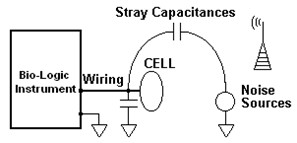
Figure 1: Stray capacitances are related to wiring.
A straightforward method to reduce the influence of the external noise sources is to use an earthed Faraday cage. Since the electrical capacitance of an object depends on the objects in its neighborhood, the Faraday cage will increase the stray capacitance to the ground, which may become an important consideration as the frequency increases.
A capacitive reactance decreases as the frequency (or pulse) increases (Eq. 1), which leads to an increased current flow outside the cell. Therefore, it may affect the accuracy of fast signal transitions and high frequency impedance measurements:
$$Z_\text C = \frac{1}{j\omega C} \tag{1}$$
In slow variation signals or low frequency conditions, the influence of the stray capacitance is insignificant and can be ignored. Note that a stray capacitance cannot be detected with a simple digital voltmeter.
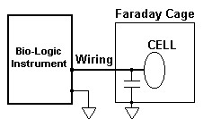
Figure 2: A Faraday Cage cut-off the noise but increase the stray capacitance to the ground.
Is there a way to evaluate the stray capacitance, for a simple interconnecting wire, for example? Well, from the electromagnetism laws [1], we know that a straight cylindrical wire manifests self-inductance and capacitance given by the following equations:
$$L/\mu \text {H }= 0.2h\left[\ln\left(\frac{4h}{d}-0.75\right)\right] \tag{2}$$
$$C/\text{pF} = \frac{h}{0.044\ln\left(\frac{4h}{d}-0.75\right)}\tag{3}$$
where d and h are the diameter and length of the wire in meters, L the inductance in µH, and C the capacitance in pF.
A 1 mm diameter wire, for example, exhibits about 1.46 µH inductance and 3.12 pF capacitance per meter. This is what theory indicates for a single straight wire. In practice, the situation is much more complicated for different reasons: interconnecting wires are placed in the vicinity of other objects grounded or not, leads ends with banana plugs which are not simple straight wires, diameter and length of leads can change to adapt further experimental requirements. For a given interconnection length, we expect the capacitance to be larger than for a same length straight wire. The best way to estimate the stray capacitance of the experimental set-up is to do an impedance measurement in the air or on a well-known dummy cell whose impedance is close to that of the studied electrochemical cell.
An example of the influence of the stray capacitance on impedance measurements is shown in Figure 3. Tests were run as an example on a VMP3 outfitted with a low current option. Counter and reference leads were stuck together (CA1, REF3 and REF2) as well as the working and sense lead (CA2 with REF1).
(Note: for VMP-300 technology, REF1, REF2, REF3, CA1 and CA2 are S1, S2, S3, P1 and P2, respectively.)
The VMP3 low current probe was placed in the middle of a 40 x 20 x 60 cm earthed Faraday cage. Three impedance tests were carried out in potentiostatic mode from 100 kHz to 0.1 Hz with 0.5 V amplitude:
A – no cell,
B – a simple 10 cm length 0.5 mm diameter wire hanging from the counter and reference,
C – same as B but the wire ends with a 4 mm banana plug.
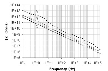
Figure 3: Impedance data A: no cell, B: 10cm wire, C: 10 cm wire + 4 mm banana plug.
All the plots are consistent with a capacitive behavior. Analysis tool like ZFit (available in EC-Lab® and EC-Lab Express software) gives a stray capacitance of 0.12 pF for “no cell” data, 0.98 pF for the 10 cm wire alone, and 2.1 pF when a banana plug is attached to the wire. If we subtract the “no cell” 0.12 pF capacitance, that should correspond to the electrometer input capacitance, we find 0.86 pF for the 10 cm wire capacitance that, as expected, is more than the theoretical value because of the grounded metallic objects in the surrounding area. Also by subtraction, we find that the 4 mm banana plug adds 1.12 pF to the wiring.
What does this mean? These tests simply illustrate that stray capacitance can affect the accuracy of high impedance samples at high frequencies. For example, for frequencies over 10 kHz, the measured impedance of a 10 MΩ resistor with 10 cm of wiring will correspond to the stray capacitance reactance and not to the value of the resistor.
LOW IMPEDANCE SAMPLES
We have seen that stray capacitance must be considered for high impedance samples at high frequencies. Low impedance samples are not at all concerned with the stray capacitances since the stray capacitance is somehow in parallel with the sample. On the other hand, the stray inductances should be seen in series with the sample and have to be carefully analyzed since they are the origin of the most perturbing factors at high frequencies.
Like stray capacitance, stray inductance is related to wiring. Obviously from Eq. 2, any piece of wire exhibits inductance. This also includes the physical dimensions of your cell. Typically, impedance measurements carried out on cylindrical batteries show an inductive effect at high frequencies. Replacing the battery by a wire of the same length will generally give the same imaginary part values at frequencies over 10 kHz.
According to the expression of the inductance impedance, an inductance will oppose more and more to the current flow as the frequency increases:
$$Z_L = j\omega L \tag{4}$$
For instance, a 10 cm length and 1 mm diameter wire has about 146 nH of inductance that, at 100 kHz, results in a 92 mW of reactance.
For example, an impedance test run with a VMP3 in galvanostatic mode with 200 mA amplitude on a 10 cm wire is shown in Fig. 4. The wire was placed between the reference shorted to the counter (CA2, REF3 and REF2) and the working (CA2 with REF1) leads.
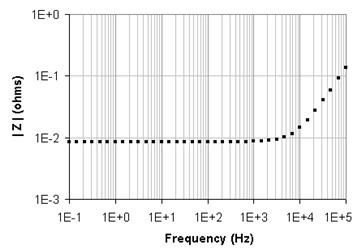
Figure 4: Impedance data for a straight 10 cm wire.
The plot confirms an inductive behavior. The best numerical fit corresponds to a 202 nH inductance in series with an 8.5 mW resistance. Besides the self-inductance of the wiring, a variable magnetic field can also corrupt EIS measurements taken on low impedance samples. Basic electromagnetism laws demonstrate that every variable current flowing through a wire creates a variable magnetic field around the wire and that a variable magnetic field induces an electromotive force in a loop (Faraday’s law):
$$E_\text{mf} = -\frac{\Delta B\,A}{\Delta t} \tag{5}$$
where ΔB is the magnetic field variation during the Δt time and A is the area of the loop.
The cables connecting the cell to the instrument have two current leads, which drive the cell current, and two potential sensing leads through which no (or a very small) current flows. The variable cell current flowing through the current leads will create a variable magnetic field that will induce a voltage in the potential sensing leads. This is the magnetic coupling effect that may appear as a fake positive or negative inductance in series with the analyzed sample:
$$Z_\text {meas} = Z_\text {real} ± j\omega L\tag{6}$$
The sign depends on the direction of the magnetic field through the loop area (Figure 7).
Several tests have been carried out to illustrate the magnetic coupling effect. On a VMP3 cable, the current leads (CA1 and CA2) and the voltage sensing leads (REF1 and REF2) have to be shortened together, in pairs, and then brought to a common point, as in Figure 5.
Although the REF3 lead does not have any contribution to the measurement, it should be connected either to the ground lead or together with REF1 and REF2 to avoid error messages with the EC-Lab® software.
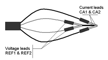
Figure 5: Magnetic coupling set-up.
Measurements have been carried out with a VMP3 in galvanostatic mode with 200 mA amplitude from 100 kHz to 0.1 Hz on the 1 A current range. The result of the experiment may look like Figure 6 and Figure 7.
The shapes of these curves show the inductive effect of the magnetic coupling. When the current leads are far from each other and the voltage sensing leads are spaced out, in other words when the induced loop area is maximized, the coupling effect is amplified (not twisted cables curves in Figure 6). The numerical fit for a LR series model gives: 145 nH for the inductance and 50 µW for the resistance. The magnetic coupling induces a constant positive or negative 90° phase shift at high frequencies. As stated above, the sign of the phase shift depends on the direction of the magnetically induced current.
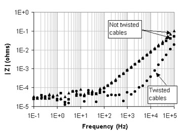
Figure 6: Magnitude spectra of the magnetic coupling.
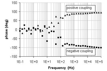
Figure 7: Phase spectra of the magnetic coupling.
Reducing both the magnetic field by twisting together the current leads and the induced loop area by twisting together the sense leads helps to minimize the magnetic coupling (twisted cables curve in Figure 6). The magnetic coupling that can be seen, even with twisted cables, should be some residual coupling equivalent to a series inductance of about 25 nH.
It should also be noted that external variable magnetic fields can induce voltages in the sense leads. Voltage can also be induced by a static magnetic field if the cell connection vibrates or simply moves.
Conclusion
Generally, impedance data can easily be misinterpreted when low or high impedance cells are measured at high frequencies. To improve the accuracy of measurements, special care must be taken with regards to cell design, connections and cell environment. High impedance cells are more sensitive to stray capacitance while low impedance cells are more sensitive to stray inductance.
Placing the cell inside a large, earthed Faraday cage can reduce the stray capacitance.
Wiring should be kept as short and small as possible to reduce both stray capacitance and stray inductance.
The magnetic coupling effect can be reduced by twisting the current leads (reducing the magnetic field) and by twisting the sense leads (reducing the induced loop).
For most part, in any application, these errors are not very important. However, a perfect understanding of the limitations of measurements is the key for a correct interpretation of the results. When making precise measurements close to limit conditions, one should be aware of sources that contribute to errors in measurements. The remaining source of errors should be taken into account when estimating the measurement uncertainty.
Although this document focuses on common sources of errors in impedance measurements, there is no reason not to consider them for other electrochemical techniques. EIS, quite simply is a technique that “exhibits” all the imperfections of a measurement set-up which are very often accentuated by the desire to go to high frequencies.
References
- F. W. Grover, in: Inductance Calculations. Princeton, NJ: Van Nostrand (Ed.), (1946). Reprinted by NY: Dover Publications (1962).
Revised in 07/2018


