

Supercapacitors Investigations Part II: Time Constant (EIS characterization) Supercapacitor – Application Note 34
Latest updated: July 31, 2023Abstract
The performances of a supercapacitor are mainly determined by the electrode material. The determination of the supercapacitor characteristics can be performed using many electrochemical techniques. In this note, an EDLC capacitor was characterized using EIS, potential pulse and potentiodynamic investigations. Two equivalent electrical circuit models at low and high frequencies were proposed. The diffusion coefficient of the electrode material was measured. The capacitance, time constant and the equivalent resistant were also determined.
Introduction
To complete the characterization performed on supercapacitors and described in application note #33 [1], it is important to define the time constant of the supercapacitor.
In this note we will describe how the supercapactor’s time constant will be determined by potentiostatic/dynamic and Electrochemical Impedance Spectroscopy (EIS) techniques.
Note that in this note (if not indicated):
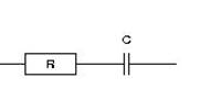
- the supercapacitor is modeled by a resistor and capacitor in series (Fig. 1).
- supercapacitor is considered as a capacitor and not as a Constant Phase Element [2].

Figure 1: Supercapacitor model
Noteworthy that time constant is similar in charge or in discharge.
Set-up description
The investigations were performed with a VMP3 equipped with a standard board. This board has EIS capability and can be connected if necessary to a 4A booster according to the needed current range.
The characteristics of the supercapacitor are described below:
capacitance: 22 F ± 30%
maximum operating voltage: 2.3 V
mass of active material: ~10 g
Supercapacitor is connected to VMP3 via a standard 2-electrode connection.
Potentio technique
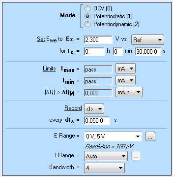
The potential pulse from 2.1 V to 2.3 V is carried out with the Modular Potentiostatic technique (Fig. 2).

Figure 2: Potentiostatic settings window.
The supercapacitor’s response to a potentio pulse follows the relationships:
$$i(t)=\frac{\left(\Delta E\right)}{R}exp\left(\frac{-t}{\tau}\right);\tau=R \tag{1}$$
Where i is the current, ΔE is the potential step, R is the resistance in series, t is the time and τ is the time constant.
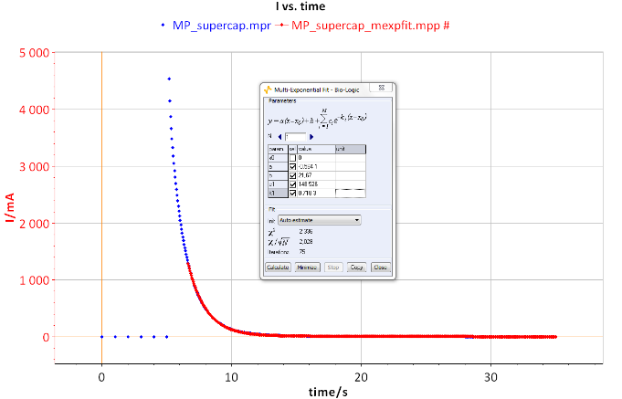
The current versus time equation is fitted with the Multi-Exponential Fit tool (Fig. 3). The time constant of the supercapacitor is 1.348 s. Moreover, it is possible to calculate the value of the series resistor of the capacitor.
At t = 0, the equation is:
$E = R I$
so,
R = 0.2 V / 4.54 A = 44.1 mΩ

Figure 3: I vs. t curve.
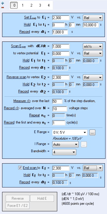
The results of the previous potentiostatic technique can be completed by a potentiodynamic one. According to the relationship I = C dE/dt, it is indeed possible to determine the capacitance of the super-capacitor at different scan rates. Potentio-dynamic investigations are carried out at several potential scans 1, 3, 10, 50 and 150 mV/s between 0 to 2.3 V. These steps are performed within the same CVA technique with the addition of sequences (Fig. 4).

Figure 4: Settings of CVA window.
The rectangular shape of the CV indicates reversible capacitive behavior (Fig. 5). When the scan rate increases, this shape evolves into a smoother rectangular shape [3,4].
The capacitance is summarized in Tab. I. Capacitance decreases when scan rate increases. The capacitance value is in the range of 25-28 F in agreement with the specification given by the manufacturer.

Figure 5: Potentiodynamic curves of supercapacitor at scan rates of 1, 3, 10, 50 and 150 mV/s.

Table I: Capacitance data.
| dE/dt (mV·s-1) | 1 | 3 | 10 | 50 | 150 |
|---|---|---|---|---|---|
| Current/mA | 28 | 80 | 262 | 1276 | 3772 |
| C/F | 28 | 27 | 26 | 26 | 25 |
EIS investigations
Time constant can also be determined by EIS investigations. Experiments are carried out in similar conditions those previously stated i.e. the same potential range. Measurements are carried out between 10 mHz to 200 kHz (Fig. 6) at several states of charge between 2.1 and 2.3 V. The Nyquist plot is shown in Fig. 7.

Figure 6: EIS settings window.
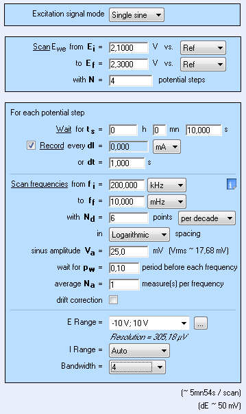

Figure 7: EIS measurements, full diagram.
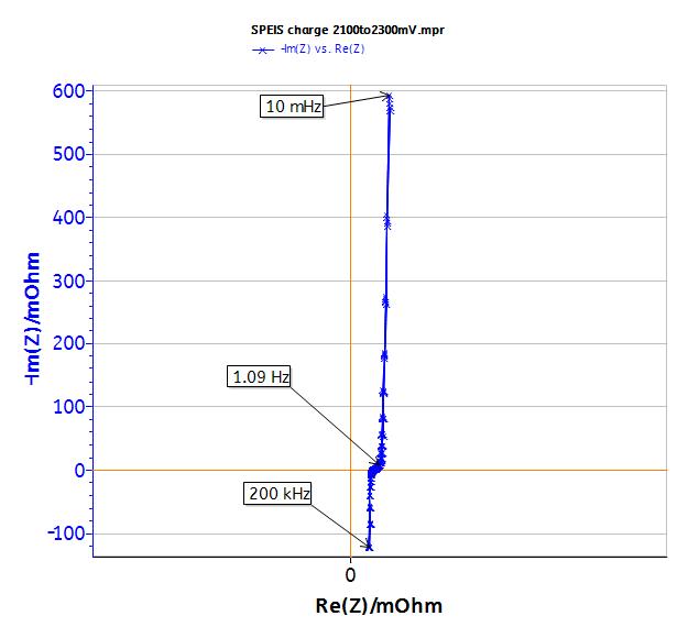
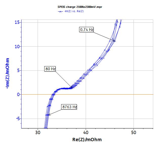
Figure 8: EIS measurement: zoom at high frequencies.
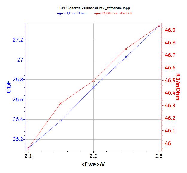
If the equivalent circuit is R + C and the fit is performed at low frequencies, Fig. 9 shows that R and C increase during the charge. Meaning that time constant increases. Please refer to application note #45 to learn how to fit multiple EIS cycles and obtain the data plot in Fig. 9.
For example, R is 52 mΩ at 2.1 V and C is 26.7 F, so τ is equal to 1.388 s. These values of R and τ are in agreement with the values previously determined by the potentio methods (Tab.II).
Figure 9: Values of the fit at low frequencies.
R, C values and time constant determined by potentio method an EIS technique are in agreement.
Table II: Capacitance measured by different methods.
| R/mΩ | C/F | τ/s | |
| Potentio | 44 | 25-28 | 1.348 |
| EIS | 52 | 26.7 | 1.388 |
At higher frequency, the simple model RC in series is no more relevant (Fig. 8). The change of the signal from 45° to 90° is indeed observed at 1 Hz. This change was already described in the literature [5-7]. This behavior cannot be modeled by the simple R + C model in series but R1+L1+C2/(R2+M2) equivalent circuit (Fig. 10). In that circuit, R1 is the internal resistance, L1 is the inductance related to the connection, R2 is the charge transfer resistance and M is due to the matter transport in thin layer in linear symmetry. The resulting curve is plotted in Fig. 10. More information is available in the impedance handbook [8].

Figure 10: Model for higher frequencies.
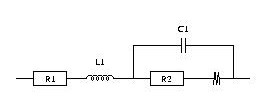
For your information, the fitted values are the following:
R1 = 31.61 mΩ
L1 = 98.45 nH
C2 = 15.59 mF
R2 = 4.23 mΩ
Rd2 = 37.89 mΩ
τd2 = 1.044 s
Note: capacitance can be determined by the ratio of τd2/Rd2 = 27.9 F.
Figure 10: Fit at high frequencies measured (x) and fitted (▼) curve.
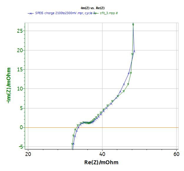
Moreover, analysis of the higher frequency data allows users to determine the diffusion coefficient thanks to the following relationship where fk is « knee » frequency and δD is the thickness between the two electrodes [8]:
$$2\pi f_k=\frac{3.88}{\left(\frac{\delta_D^2}{D}\right)} \tag{2}$$
Conclusion
This note shows how to determine the time constant by DC potentio and EIS techniques. The EIS method is more powerful because additional high frequency information is available.
Data files can be found in :
C:\Users\xxx\Documents\EC-Lab\Data\Samples\Supercapacitor\technique_supercap
References
1) Application note 33 “Supercapacitors investigations. Part I: charge/discharge cycling”
2) Application note 21 “Measurements of the double layer capacitance”
3) F. Moser, L. Athouël, O. Crosnier, F. Favier, D. Bélanger, T. Brousse, Electrochem. Communications, 11 (2009) 1259.
4) P. Ragupathy, H. N. Vasan, N. Munichandraiah, J. Electrochem. Soc., 155 (2008) A34.
5) A. J. Roberts, R. C.T. Slade, Electrochim. Acta, 55 (25) (2010) 7460.
6) V. Ruiz, C. Blanco, R. Santamaria, J. M. Ramos-Fernandes, M. Martinez-Escandell, S. Sepulveda-Escribano, F. Rodriguez-Reinoso, Carbon, 47 (2009) 195.
7) P. L. Taberna, P. Simon, J. F. Fauvarque, J. Electrochem. Soc., 150 (2003) A292.
8) Handbook of Electrochemical Impedance Spectroscopy. DIFFUSION IMPEDANCES – [PDF]
Revised in 08/2019


