

CASP: a new method for the determination of corrosion parameters (CASP Rp determination) Corrosion – Application Note 37
Latest updated: July 17, 2024Abstract
The Constant Amplitude Sinusoidal microPolarization (CASP) technique is an innovative protocol for the determination of corrosion parameters with EC-lab software. In this note, the theory and the equations involved in the CASP technique were introduced. The results of the characterization of Nickel in acidic media using CASP are given here. The results were also compared with the corrosion rate and Tafel parameters obtained with Tafel Plot technique. It was shown that the corrosion parameters obtained with VASP technique are similar to those obtained with Tafel plot technique with a significantly shorter time and less disturbance of the corrosion system.
Introduction
The steady-state current vs. potential characteristic I vs. E of a metal with a corrosion potential $I_\text{corr}$ is given by the Stern
$$I=I_\text{corr}\exp{\left(\frac{\ln{1}0\left(E-E_\text{corr}\right)}{\beta_\text a}\right)}\ -I_\text{corr}\exp{\left(\frac{-\ln{1}0\left(E-E_\text{corr}\right)}{\beta_\text c}\right)} \tag{1}$$
Where $I_\text{corr}$ is the corrosion current of the considered metal and $\beta_\text a$ and $\beta_\text c$ the Tafel parameters.
Two classical methods based on the Stern relation are commonly used to determine the uniform corrosion current $I_\text{corr}$ of a metal in contact with an aggressive solution:
- Using the Tafel method [1], which requires the application of significantly large overpotentials (typically over +/-100 mV).
- Determining the polarization resistance $R_\text p$ [1] by applying a small sinusoidal potential perturbation and using the Stern-Geary relation, which requires knowledge of Tafel parameters.
For a low enough frequency, the relation (1) can be used to describe the current response and lead to the corrosion parameters, $I_\text{corr}$ and the Tafel parameters $\beta_\text a$ and $\beta_\text c$. This is the basis of the CASP (Constant Amplitude Sinusoidal microPolarization) technique.
In this note, first of all, the theory and the equations involved in the CASP technique are introduced. Secondly, the configuration of EC-Lab® for CASP measurements is described. Finally, a short comparative study of the results with the Tafel Fit method is presented.
Theoretical background
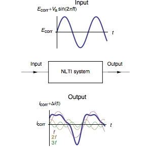
The CASP method analyzes the response of an electrochemical system subjected to a sinusoidal potential of constant amplitude and frequency.
This sinusoidal voltage of amplitude $V_\text a$, of frequency $f$ applied around the corrosion potential $E_\text{corr}$, is expressed as:
$$\Delta E(t)=E(t)-E_\text{corr}=V_\text a \sin{(2\pi ft)} \tag{2}$$
For a system in which the electrolyte resistance $R_\Omega $ is negligible compared to the polarization resistance $R_\text p$
$$I(t)=I_\text {corr}\left(\exp{\left(\frac{\ln{10}\,V_\text a\sin{(2\pi ft)}}{\beta_a}\right)}\ -\exp{\left(\frac{-\ln{10}\,V_\text a\sin{(2\pi ft)}}{\beta_c}\right)} \right)\tag{3}$$
The Fourier series expansion of the expression (3) shows that $I(t)$ is expressed as a sum of sine waves, one at the fundamental frequency $f$ and the other at frequencies that are an integer multiple of the fundamental frequency, called harmonics (Fig. 1).

Figure 1: Current response of a Non-Linear Time Invariant (NLTI) system subjected to sinusoidal voltage perturbation.
The number of apparent harmonics depends on the amplitude of the sinusoidal potential. In CASP Fit, only the first three harmonics are used. Their amplitudes $\delta I_1$, $\delta I_2$, $\delta I_3$ are determined and used in (4-6) to determine the corrosion current and the parameters $b_\text a$ and $b_\text c$ with $b_\text {a,c} = \ln 10/\beta_\text {a,c}$. The Fourier expansion and more details about relations (4-6) can be found in [2-4].
$$I_\text{corr}=\frac{1}{4\sqrt3}\frac{\left(\delta I_1+3\delta I_3\right)^2}{\sqrt{\left|\delta I_2^2+2\delta I_3\left(\delta I_1+3\delta I_3\right)\right|}} \tag{4}$$
$$b_\text a=\frac{2}{\delta E}\frac{\sqrt3\sqrt{\left|\delta I_2^2+2\delta I_3\left(\delta I_1+3\delta I_3\right)\right|}-\delta I_2}{\delta I_1+3\delta I_3} \tag{5}$$
$$b_\text c=\frac{2}{\delta E}\frac{\sqrt3\sqrt{\left|\delta I_2^2+2\delta I_3\left(\delta I_1+3\delta I_3\right)\right|}+\delta I_2}{\delta I_1+3\delta I_3} \tag{6}$$
Experimental parameters
Choice of the frequency
The impedance of the system at the chosen frequency should be close to $R_\text p$. An impedance Nyquist diagram of the electrode in the electrolyte of interest is needed to determine this frequency. Details on impedance measurements and Nyquist diagram can be found in [5,6].

Figure 2: Parameters used for the preliminary impedance measurement.
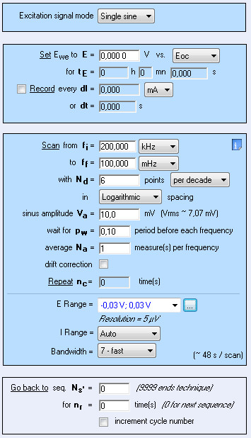
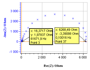
The system chosen is a 99.9 % pure Ni 1 mm diameter wire immersed in 0.5 mol·L-1 H2SO4. The surface exposed is 0.72 cm2. All potentials are given vs. Ag/AgCl reference electrode. The impedance measurement was performed using an SP-200 and the chosen parameters are shown in Fig. 2. The resulting Nyquist diagram is shown in Fig. 3. Assuming that the equivalent circuit is an R/C circuit, $R_\text p$ is measured at the frequency for which Im(Z) → 0 at low frequencies. In Fig. 3, this frequency is 0.1 Hz. This value is low enough to consider that the voltage perturbation is steady-state. It is a common value for a corroding metal and is set as a default value in EC-Lab® . It can be seen in the impedance graph (Fig.3) that the electrolyte resistance $R_\Omega$ (Z for Im(Z)→0 at high frequencies) is negligible compared to $R_\text p$: 16.4 Ω and 6270 Ω, respectively.

Figure 3: Nyquist diagram of the impedance of the Ni electrode in 0.5 mol·L-1 H2SO4.
Choice of the amplitude
As noted above, Eq. (4-6) are written using the first three harmonics. $V_\text a$ must be large enough so that the amplitude of the third harmonic is around 1 or 2 % of the amplitude of the fundamental harmonic and small enough so that the fourth harmonic does not appear [2]. Examples will be shown below.
EC-LAB®/EC-LAB® Express configuration
The CASP method is available in the Corrosion applications section. The settings are shown in Fig. 4. It is possible to adjust the duration of the sinusoidal perturbation by setting the number of periods (Fig. 4).

Figure 4: CASP settings.
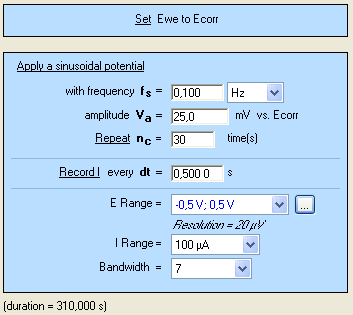
A high number of repetition will ensure a high number of points providing a better average of the harmonics’ amplitudes. $E_\text{range}$ must be set as small as possible as it will improve the accuracy of the applied potential. The same rule applies to $E_\text{range}$ as it will increase the accuracy of the measured current.
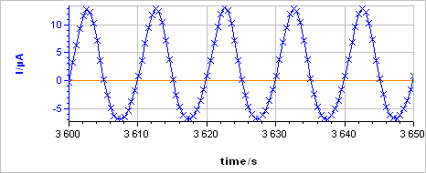
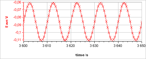
The sample was left immersed in the solution during 1 h before the measurement. The raw output is a current vs. time trace shown in Fig. 5a corresponding to the voltage perturbation shown in Fig. 5b. At 0.1 Hz the impedance has only a real part (Im(Z) = 0) so there is no phase shift between $I(t)$ and $E(t)$.

Figure 5: a) Current response from b) voltage perturbation obtained using settings shown in Fig. 4.
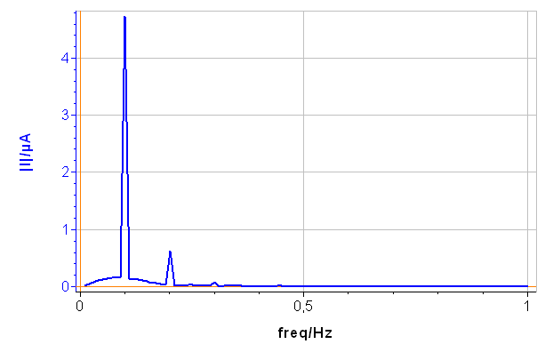
The CASP Fit tool is located in the Corrosion Analysis tools. It performs a Discrete Fourier Transform (DFT) of the current versus time trace, determines the amplitudes of the harmonics and calculates the corrosion parameters $I_\text{range}$, $\beta_\text a$ and $\beta_\text c$. The amplitude spectrum and analysis are shown on Figs. 6a and 6b, respectively.
Results
CASP Fit
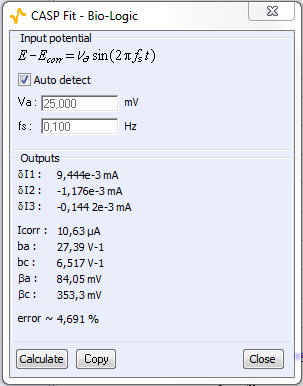
In Fig. 6, a), the tree harmonics appear, which show that the chosen amplitude $V_\text a$ was appropriate. The amplitude of the third harmonic at 0.3 Hz represents 1.5% of the amplitude of the fundamental frequency, which shows that the chosen amplitude $V_\text a$ was not too small. In Fig. 6, b), the amplitudes $\delta I_2$, $\delta I_3$ are negative, which is generally the case for the corroding materials in acidic and neutral electrolytes. The analytically calculated values $I_\text{corr}$, $\beta_\text a$ and $\beta_\text c$ as well as $\beta_\text a$ are also shown. The corrosion current is 10.6 µA corresponding to a corrosion current density of 15 µA cm-2. It is the same order of magnitude as the value obtained by Sato [7].


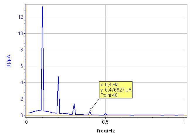
Figure 6: a) Amplitude spectrum of the current res ponse shown in Fig. 5a), b) Corresponding CASP Fit results
The results shown in Fig. 7 were obtained on pure Ni in 0.5 M H2SO4 with an amplitude $V_\text a$ of 75 mV. The fourth harmonic at 0.4 Hz can be seen, showing that the applied amplitude, i.e. 75 mV, must be reduced.

Figure 7: Amplitude spectrum of a current response obtained with a voltage amplitude $V_\text a$ of 75 mV.
Comparison with the tafel method
A polarization curve was obtained using the Linear Polarization (LP) technique with the same parameters as in ASTM G5 (Standard Reference Test Method for Making Potentiostatic and Potentiodynamic Anodic Polarization Measurements) [8].

Figure 8: Linear polarization (LP) settings
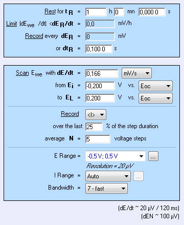


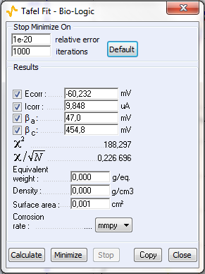
Figure 9: a) Polarization curve obtained with settings shown in Fig. 8, b) corresponding Tafel Fit results
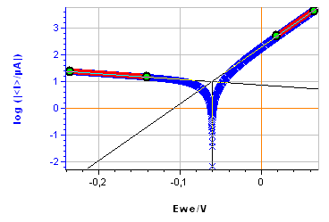
The sample was left immersed in the solution during 1 h before the measurement. The parameters for the linear polarization, the corresponding curve and the Tafel Fit analysis are shown on Figs. 8, 9a and 9b, respectively.
Table I shows the values and the relative difference for $E_\text{corr}$, $\beta_\text a$ and $\beta_\text c$ obtained with CASP Fit and Tafel Fit. The values used were averaged from three different experiments performed in the same conditions. There is a good agreement between both methods for the determination of $E_\text{corr}$.
Table I : Comparison of the Tafel Fit and the CASP Fit
| Parameter | Icorr/µA | βa/mV | βc/mV |
|---|---|---|---|
| CASP Fit | 10.6 | 84,05 | 353.3 |
| Tafel Fit | 9.85 | 47 | 455 |
| Relative difference/% | 7 | 44 | 19 |
There is a decent agreement for $\beta_\text c$. For both methods, the $\beta_\text c$ value is large, indicating that the cathodic reaction is limited by mass transport, which can be seen on the current-potential characteristic (Fig. 9a).
The two main advantages of the CASP technique are that:
- It is a faster technique. The CASP measurement took only around 5 min for 30 cycles (Fig. 4) whereas the LP for the Tafel fit took 40 min (400 mV was scanned for a scan rate of 10 mV/min).
- It is less disturbing for the system.

Figure 10: Evolution of the corrosion potential after a linear polarization with the settings shown in Fig. 8 and after a CASP measurement with the settings shown in Fig. 4.
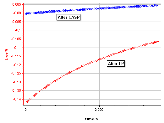
Figure 10 compares the evolution of the corrosion potential of pure Ni in 0.5 mol·L-1 H2SO4 after the LP and after the CASP. After LP, the potential increases from -0.142 to – 0.106 V vs. Ag/AgCl, due to repassivation of the Ni surface after anodic depassivation. After CASP, the potential increases only from -0.090 to -0.085 V vs. Ag/AgCl. $I_\text{corr}$ is also available in CASP as it is the potential around which the voltage perturbation is applied. It can be read on the potential vs. time trace (Fig. 5b).
Conclusion
Available in EC-Lab®, CASP is a new way to obtain the corrosion current and the Tafel parameters of a corroding system. This technique is based on the analysis of the current response of a non-linear electrochemical system subjected to a sinusoidal voltage perturbation. An impedance measurement is recommended before the CASP technique to obtain the best frequency for the voltage perturbation. CASP Fit gives the same corrosion current as Tafel Fit but in a significantly shorter time and with much less disturbance of the electrochemical system.
Data files can be found in :
C:\Users\xxx\Documents\EC-Lab\Data\Samples\Corrosion\X_CASP
References
1) Application Note #10 “Corrosion current measurement for an iron electrode in an acid solution”
2) L. Mészáros et al., J. Electrochem Soc., 141 (1994) 2068.
3) J.-P. Diard et al., J. Electrochem Soc. Comments, 142 (1995) 3612.
4) C. Montella, J.-P. Diard, B. Le Gorrec, Exercices de cinétique électrochimique, Hermann, Paris, 164 (2005) 270.
5) Application note #8 “Impedance, admittance, Nyquist, Bode, Black, etc…”
6) Application note #14 “ZFit and equivalent electrical circuits”
7) N. Sato et al., J. Electrochem. Soc., 110 (1963) 605.
8) ASTM G5-94, ASTM Publications
9) C. Wagner, R. Traud, Corrosion NACE, 62, 10 (2006) 843.
Revised in 08/2019


