

ZFit and equivalent electrical circuits (EIS Equivalent Circuit) Battery – Application Note 14
Latest updated: November 28, 2023Abstract
This application note explains the general approach to fitting an Electrochemical Impedance spectrum, to an equivalent circuit. After a spectrum is recorded, an equivalent circuit can be picked from the list of pre-programmed circuits, or built by the user with the ‘Edit’ tool. Extra attention has to be paid to pick a circuit that appropriately represents the physical model of the sample under study. Often times different circuits can match the electrical response of the sample, but only one will correspond to its material characteristics (for example two different ladder models, Voigt or Maxwell). Values obtained with different models can be transformed using appropriate formulae.
Introduction
It is well documented that different electrical circuits can explain EIS data in an equivalent manner, that is, they exhibit identical impedance for all frequencies [1-4].
EC-Lab® software is provided with a powerful tool for EIS data analysis called ZFit. This tool can perform electrical circuit identification with EIS experimental data files obtained with either Bio-Logic potentiostat/galvanostat or with other systems on the market. In fact, EC‑Lab® software can import ASCII text files generated by other electrochemical stations and perform efficient EIS fits. The user can choose between two different minimization algorithms, Simplex and Levenberg-Marquardt, to achieve the best electrical element values.
The aim of this note is to explain how to fit EIS data with EC-Lab® software and show the user equivalent circuits that can fit the same EIS data file in particular conditions.
Fitting an Experimental Nyquist Impedance Diagram Using ZFit
The Nyquist impedance diagram shown in Fig. 1 has been measured for circuit #3 of the BioLogic test-box 3 using the PEIS protocol. Test circuit #3 mainly consists of two transistors. It is a model for metal passivation [5]. The Nyquist impedance diagram shown in Fig. 1 is made of two capacitive arcs well separated in frequency.
It is possible to load the PEIS_0‑8V_circuit3.mpr file with EC-Lab® software in the following folder: C\EC‑Lab\Data\Samples.
Let us suppose that the Nyquist impedance diagram shown in Fig. 1 has been obtained for an electrochemical system, and we want to characterize this electrochemical impedance diagram with an electrical circuit.
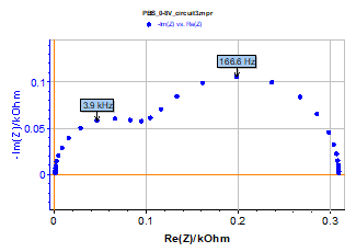
Figure 1: Test circuit #3. Nyquist impedance diagram measured using PEIS technique. EWE= 0.8 V, Va= 0.8 V, fmin= 1 Hz, fmax= 100 kHz.
The electrical circuit shown in Figure 2 is first selected because it matches the Faradaic impedance structure for an electrochemical system with R1 = Rct and C1 = Cdl where Rct is the charge transfer resistance, and Cdl the double layer capacitance. The corresponding Equivalent Circuit Edition window is shown in Figure 3.
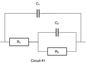
Figure 2: Equivalent circuit #1 made of two resistors and two capacitors. Ladder circuit C1/(R1+C2/R2).
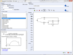
Figure 3: Equivalent Circuit Edition window. Ladder circuit C1/(R1+C2/R2).
Clicking in the boxes for the elements and their numbers in the Equivalent Circuit Edition window makes it easy to choose an electrical circuit. The results of the ZFit procedure using Randomize + Levenberg-Marquardt are shown in Figure 4.
Equivalent Electrical Circuit
ZFit indicates known equivalent circuits in the description window (Figure 3).
Three others circuits shown in Figure 5, made of two Rs and two Cs, can be used to characterize the Nyquist impedance diagram shown in Figure 1. It is very easy, using ZFit, to verify this quite surprising result, sometimes ignored by electrochemists.
The results of the ZFit procedure using Randomize+Levenberg-Marquardt for the three circuits shown in Figure 5 are given in Figure 6 to Figure 8. The sums of square of residuals, χ², are very closed for the four circuits, with χ²/|Z| ~ 1.44. The four circuits are therefore indistinguishable, and all of them can be used to characterize the Nyquist impedance diagram shown in Figure 1.
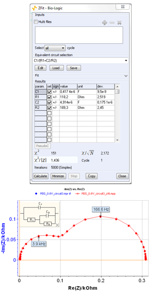
Figure 4: ZFit window for circuit #1. Ladder circuit C1/(R1+C2/R2).
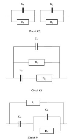
Figure 5: Three electrical circuits made of two Rs and two Cs equivalent to circuit #1. Circuit #2: Voigt circuit C1/R1+C2/R2), circuit #3: Maxwell circuit C1/R1/(C2+R2), circuit #4: ladder circuit R1/(C1+R2/C2).
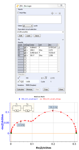
Figure 6: ZFit window for circuit #2: Voigt circuit C1/R1+C2/R2.
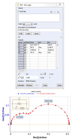
Figure 7: ZFit window for circuit #3: Maxwell circuit C1/R1/(C2/R2). Figure 8: ZFit window for circuit #4: ladder circuit R1/(C1+C2/R2).
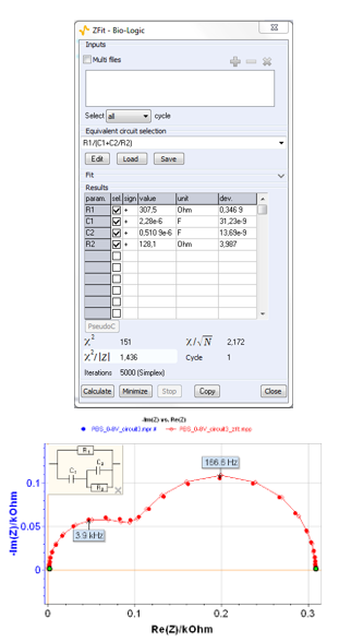 Figure 8: ZFit window for circuit #4: ladder circuit R1/(C1+C2/R2).
Transformation Formulae
The common structure of the impedance circuits #1-4 is written as:
$$Z(f) = \frac{K(1+\tau_1\ j2\ \pi f)}{(1 + \tau_2\ j2\ \pi f)+(\tau_3\ j2\ \pi f)^2} \tag{1}$$
It is therefore possible to write algebraic relationships used to determine transformation formulae. As an example, the simplest transformation formula are obtained for circuit #1 and #3 [4]:
$$C_{13} = C_{11},\, R_{13} = R_{11} + R_{21} \tag{2}$$
$$C_{23} = \frac{C_{21}R_{21}^{2}}{(R_{11}+R_{21})^2} \tag{3}$$
$$R_{23} = \frac{R_{11}^2}{R_{21}}+R_{11} \tag{4}$$
where the second subscripts denote the rank of the circuit. Using these transformation formulas with best fit parameter values obtained for circuit #1 (Fig. 4) and calculating value for circuit #3, it is obtained:
$C_{13} = 4.17·10^{-7}\ F,\ R_{13} = 307.5\ \Omega$
$R_{23} = 192.0\ \Omega,\ C_{23} = 1.86·10^{-6}\ F$
These parameter values are very close to the best fit parameters value obtained using ZFit for circuit #3 (Figure 7):
$C_{13} = 4.17·10^{-7}\ F,\ R_{13} = 307.5\ \Omega$
$R_{23} = 191.9\ \Omega,\ C_{23} = 1.86·10^{-6}\ F$
Analogous relationships can be obtained with the others circuits [4].
Conclusion
In this note, we have introduced ZFit, the EIS fitting tool available in EC-Lab®, and showed how it can be used to fit impedance data using electrical equivalent circuits. There are many different electrical equivalent circuits which correspond one impedance diagram. The effectiveness of the process is dependent on the ability to choose the best circuit representing the physical reality of the system being studied.
References
- I.M. Novosel’skii, N.N. Gudina, Y.I. Fetistov, Elektrokhimiya 8 (1972) 565.
- J.R. Macdonald, in: Impedance spectroscopy, Wiley, New York (1987).
- S. Fletcher, J. Electrochem. Soc., 141 (1994) 1823.
- F. Berthier, J.P. Diard, R. Michel, J. Electroanal. Chem., 510 (2001) 1.
- Application Note #9 “Linear vs. non linear systems in impedance measurements”
Revised in 07/2018


