An investigation of corrosion kinetics using BioLogic’s Corr.Sim tool

Introduction

Corr.Sim is a proprietary simulation tool available in EC-Lab® software. It can be used for research purposes and in education as a teaching tool. It is also the perfect tool for self-learning – helping beginners consolidate their knowledge of electrochemistry.

Corr.Sim has been developed to help users gain a better understanding of the corrosion behavior of a material in a given environment.

The tool has been based on three relationships/three known techniques:

• The Stern relationship, a fundamental equation of electrode kinetics used for simulating Tafel plots and for Tafel fits [1]
• Variable Amplitude Sinusoidal Polarization technique (VASP) [2]
• Constant Amplitude Sinusoidal Polarization technique (CASP) [3]

All three techniques lie on the assumption that the studied system is Tafelian, that is to say, the corrosion kinetics only depend on the electronic charge transfer rate, ie the potential, following the Stern-Geary or Wagner-Traud relationship. It should be noted that the Tafel extrapolation technique can also be used in cases where the corrosion is limited by mass transport [4].

In this article, we will focus on, and review the Tafel plot simulation based on the Stern relation. This simulation allows the visualization of the corrosion processes, the understanding and the interpretation of the experimental plots.

The article is divided into two sections:

• Simulation of Tafel plots (high overpotential)
• Simulation of the polarization resistance (low overpotential)

Simulation of Tafel Plots

The corrosion behavior of a material (termed here as an electrode) in its environment can be described and investigated using Tafel plots. These curves describe the variation of current density with respect to the electrode overpotential in cases where the corrosion kinetics are only due to electronic charge transfer. They can be simulated using Corr.Sim. This simulation is based on the Stern or Wagner-Traud relation where two half electrochemical reactions from two different redox couples, are involved in the overall corrosion reaction [5]:

$$I=I_{\mathrm{corr}}\left(\exp\left(\ln{10}\frac{\eta}{\beta_\mathrm{a}}\right)-\exp\left(-\ln{10}\frac{\eta}{\beta_\mathrm{c}}\right)\right)\tag{1}\label{eq1}$$

With $\eta=E-E_{\mathrm{corr}}$ the overpotential, $E$ the applied voltage, $E_{\mathrm{corr}}$ the corrosion potential, $I$ the current, $I_{\mathrm{corr}}$ the corrosion current density, $\beta_\mathrm{a}$ and $\beta_\mathrm{c}$ are known as Tafel coefficients.

Equation $\eqref{eq1}$ can also be written as:

The Tafel coefficients are expressed as:

$$\beta_{\mathrm{a}}=\frac{RT}{n_1\alpha_\mathrm{a}F}\tag{3}\label{eq3}$$

and

$$\beta_{\mathrm{c}}=\frac{RT}{n_2\alpha_\mathrm{c}F}\tag{4}\label{eq4}$$

With $\alpha_\mathrm{a}$ the anodic transfer coefficient of the metal oxidation,  $\alpha_\mathrm{c}$ the cathodic transfer coefficient of the oxidant reduction, $F$ the Faraday constant, $R$ the perfect gas constant, $n_1$ and $n_2$, the number of electrons involved in the anodic oxidation of the metal and the cathodic reduction of the oxidant, respectively.

The theoretical relationships $\eqref{eq1}$ and $\eqref{eq2}$ assumes a uniform corrosion in which the corrosion reaction is under activation control (or electron transfer control).

At larger overpotentials, the relation $\eqref{eq2}$ can be reduced to two linear polarization curves called Tafel plots: an anodic curve with a slope of $\frac{1}{\beta_\mathrm{a}}$ corresponding to the oxidation reaction and a cathodic curve with a slope of $\frac{1}{\beta_\mathrm{c}}$ corresponding to reduction reaction.

Figure 1 shows an example of simulated Tafel plot obtained with Corr.Sim using  $I_\mathrm{corr}$, $E_\mathrm{corr}$, the $\frac{1}{\beta_\mathrm{a}}$ and $\frac{1}{\beta_\mathrm{c}}$ values shown in the setting table on the left of the Figure 1.

The red star in Fig. 1 corresponds to the intercept of the anodic and cathodic Tafel plots characterized by $\frac{1}{\beta_\mathrm{a}}$ and $\frac{1}{\beta_\mathrm{c}}$ slopes respectively. The coordinates of this point are $\log{I_\mathrm{corr}}$ and $E_\mathrm{corr}$.

Figure 1: Example of Tafel plot (right) drawn using Corr.Sim with a voltage scan of ± 250 mV
around $E_\mathrm{corr}$. Corr.Sim setting window showing the setting parameters (left).

Corr.Sim can be used to carry out a parametric study to investigate the effect of the corrosion parameters on the kinetic and the shape of Tafel plots by varying one corrosion parameter and keeping the other parameters constant. The obtained plots can be used for the prediction/forcast of the behavior of a corrosion system when the corrosion potential or Tafel parameter changes. Once a suggested corrosion mechanism suits the experimental data, Corr.Sim can be used to recheck and confirm the validity of the suggested kinetic model. Corr.Sim can also generate Tafel plots drawn using various experimental Tafel parameters reported in the literature. The simulated plots can be exported as a text file in order to be processed using a spreadsheet program like Excel, Origin, etc.

Figure 2 shows the simulated Tafel plot obtained with a fixed corrosion potential and an increased magnitude of $\beta_{\mathrm{a}}$ and $\beta_{\mathrm{c}}$.

Figure 2: Shape of Tafel plots for fixed corrosion potential and increased Tafel parameters.
Please see a summary of the Tafel method in the corresponding topic [6].

Simulation of polarization resistance

Another use of the Corr. Sim tool is the estimation of polarization resistance. The definition of polarization resistance $R_\mathrm{p}$ is:

$$R_\mathrm{p}=\frac{1}{\frac{\mathrm{d}E}{\mathrm{d}I}}\tag{5}\label{eq5}$$

Which gives, at $E= E_\mathrm{corr}$, using Eq. $\eqref{eq2}$:

$$R_{\mathrm{p},{E_\mathrm{corr}}}=\frac{\beta_{\mathrm{a}}\beta_{\mathrm{c}}}{I_\mathrm{corr}(\beta_{\mathrm{a}}+\beta_{\mathrm{c}})\ln{10}}\tag{6}\label{eq6}$$

This the Stern and Geary relationship, that allows the determination of the corrosion current by measuring polarization resistance and an understanding of the values of the Tafel parameters.

Figure 3 shows an example of a polarization curve at low overpotential obtained with Corr.Sim.

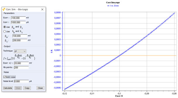
Figure 3: I vs. E curve for a low overpotential range η± 20 mV.

[1] Application Note 10:  Corrosion current measurement for an iron electrode in an acid solution

[2] Application Note 36: VASP an innovative technique for corrosion monitoring

[3] Application Note 37: CASP a new method for the determination of corrosion parameters

[4] Application Note 47:  Corrosion current determination with mass transfer limitation

[5] Tutorial: Corrosion, Part 1: Theory and basics.

[6] BioLogic topic: Corrosion basics: determination of the corrosion current and potential