

VASP: an innovative technique for corrosion monitoring (VASP Rp determination) Corrosion – Application Note 36
Latest updated: July 17, 2024Abstract
Variable Amplitude Sinusoidal micro-Polarization technique is an electrochemical protocol based on EIS measurements using low voltage amplitude perturbation. Like the Tafel plot technique, the VASP allows the determination of the corrosion rate and Tafel parameters of a corrosion system without sample surface destruction. In this note, the VASP technique is introduced. The corrosion parameters of a pure Nickel sample in acid media were determined using VASP technique. The obtained results were compared with those obtained with Tafel plot technique.
Introduction
Variable Amplitude Sinusoidal micro-Polarization technique (VASP) is a new electrochemical method integrated in EC-Lab®. It is based on an electrochemical impedance measurement that allows the study of corrosion mechanisms by the determination of Tafel parameters $\beta_\text a$, $\beta_\text c$; and the corrosion current $I_\text{corr}$.
The VASP technique consists of determining the change of the measured polarization resistance $R_\text{p}$ with the potential amplitude variation. $R_\text{p}$ is determined by Electrochemical Impedance spectroscopy measurements at a fixed and low enough frequency $f_\text{s}$. $f_\text{s}$ determination is defined in the next paragraph.
The VASP experiment is performed by applying a sinusoidal electrical potential $E_\text{WE}(t)$:
$$E_\text{WE}\left(t\right)=V_\text a \sin{(}2\pi\ f_\text st) \tag{1}$$
with variable amplitude values and by determining at the frequency $f_\text{s}$ the polarization resistance for each amplitude.
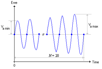
The sinusoidal potential $E_\text{WE}(t)$ is applied around open circuit potential (OCP) with amplitudes increasing from $V_\text{a min}$ to $V_\text{a max}$.

Figure 1: Sinusoidal potential $E_\text{WE}(t)$ with amplitudes increasing from $V_\text{a min}$ to $V_\text{a max}$.
Any electrochemical system is non-linear and its response depends on the input modulation amplitude. However, we can always find a low enough amplitude such that an electrochemical system can be considered linear.
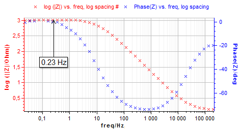
The frequency $f_\text{s}$ is previously determined by an EIS technique on a wide frequency range. The Fig. 2 shows the Bode diagram for the Nickel electrode in 0.1 mol·L-1 HCl media.

Figure 2: Bode impedance diagram for $f_\text{s}$ frequency determination.
The frequency $f_\text{s}$ is determined on the Bode plot and corresponds to the low frequency where $\text {Im}(Z)=0$ (i.e φ=0).
The electrode impedance at the frequency $f_\text{s}$ is a real parameter:
$$Z\left(f_\text s\right)=R_\text p \tag{2}$$
For negligible Ohmic drop, $R_\Omega \approx 0$, the $R_\text p$ parameter can be expressed by the following relation [1,2]:
$$\frac{1}{R_\text p}=I_\text{corr}\sum_{k=0}^{\text K}{\frac{b_\text a^{2k+1}+b_\text c^{2k+1}}{2^{2k}k!\left(k+1\right)!}V_\text a^{2k}} \tag{3}$$
Where $b_\text a$ and $b_\text c$ are the Tafel slopes:
$$b_\text a=\frac{\ln{10}}{\beta_\text a}, \, b_\text c=\frac{\ln{10}}{\beta_\text c} \tag{4}$$
The corrosion parameters are determined by numerically fitting the data with Eq. 3.
This note explains how to perform a VASP experiment. The resulting data are compared with those obtained with a Linear Polarization Resistance (LPR) test.
Experimental setup
Investigations were performed at room temperature using a SP-300 potentiostat with EIS capability.
- Working electrode: Pure Nickel wire with immersed area S = 0.6 cm².
- Counter electrode: Platinum wire
- Saturated Calomel Electrode (SCE)
- Solution: HCl (1 mol·L-1)
On the setting window of VASP (Fig. 3), the user can set the frequency value of the applied potential. The maximum and the minimum values of the potential amplitude and the number of steps N are also entered.
In this application note, the chosen settings are shown on Fig. 3. The experiment is performed at the frequency $f_\text s$ = 0.23 Hz using $N$ = 20 sinus amplitude. The frequency value $f_\text s$ was determined by the impedance measurement graph shown above (Fig. 2).

Figure 3: Setting window of VASP experiment.
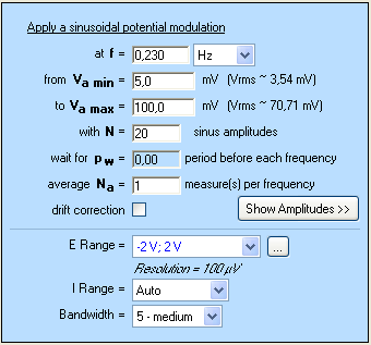
Commonly, amplitudes of applied potential are chosen between $V_\text{a min}$= 10 mV vs. OCV and $V_\text{a max}$= 100 mV vs. OCV. For $N$ measured points, the amplitude of the applied potential increases from $V_\text{a min}$ to $V_\text{a max}$ by a step of $\frac{V_{\text{a max}} – V_{\text{a min}}}{N-1}$. In our case, the potential increases by 5 mV from one point to the next one.
Results
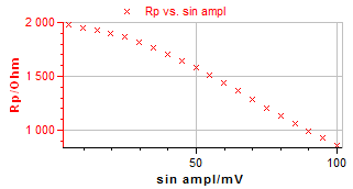
Figure 4 illustrates the VASP plot from which the corrosion current $I_\text{corr}$ and the Tafel parameters $β_\text a$ and $β_\text c$ can be estimated.

Figure 4: VASP plot.
In the Analysis/Corrosion menu the user can select the “VASP Fit” analysis. This tool allows the user to calculate the corrosion current $I_\text {corr}$ and Tafel parameters $β_\text a$, $β_\text c$.
Once the numerical fitting is launched, the simulated plot is added to the VASP plot as shown in Fig. 5.

Figure 5: VASP Fitting plot.
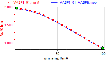

Figure 6: VASP Fit window.
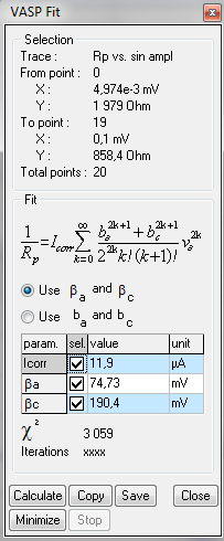
The user has the choice between $β_\text a$, $β_\text c$ parameters and $b_\text a$, $b_\text c$ Tafel slopes. These parameters can be obtained by ticking the “use $b_\text a$ and $b_\text c$” box in the VASP Fit window (Fig. 6).
The results of the VASP experiment were compared with those obtained by the linear polarization technique.
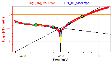
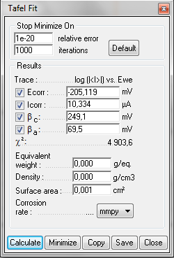
As mentioned in the application note related to the linear polarization resistance (LPR) technique [3], the “Tafel Fit” tool provides an estimation of the corrosion rate and of the Tafel parameters. Fig. 7 shows the Tafel curve and the fitting plot obtained on pure Nickel in HCl media. The estimated corrosion parameters are illustrated in Fig. 8.

Figure 7: Tafel plot.
In similar experiment conditions, both techniques should provide similar results.
A slight difference can be observed between the Fit parameter’s values obtained by LPR and VASP techniques. It may be due to differences in the surface state between the two samples.

Figure 8: Tafel Fit window.
The table below summarizes the data obtained from the two experiments. The corrosion parameters obtained from VASP technique are compared with those obtained by classical linear polarization technique. Considering the surface change, the values of the corrosion parameters obtained with both techniques are in decent agreement.
Table I: comparison between VASP and LPR parameters.
| Corrosion parameters | LPR | VASP | Deviation (%) |
|---|---|---|---|
| Icorr/µA | 10.3 | 11.9 | 13 |
| βa/mV | 69.5 | 74.73 | 07 |
| βc/mV | 249.1 | 190.4 | 23 |
Conclusion
This application note presented the use of the VASP technique integrated to EC-Lab® and EC-Lab Express® software. The corrosion parameters obtained from this technique are compared with those obtained by linear polarization resistance (LPR) method. It showed that the corrosion parameters fitted by VASP technique are close to those obtained by LPR technique. The VASP method is often a quickly implementable technique, easier to perform on several electrochemical systems.
Due to the low potential amplitudes, the VASP technique has the advantage of only slightly modifying the surface properties of an electrode compared to the LPR technique that alters the electrode surface. The VASP technique is recommended for potential sensitive surface electrode.
Data files can be found in :
C:\Users\xxx\Documents\EC-Lab\Data\Samples\Corrosion\PEIS_VASP, VASP_VASP and LP_VASP
References
1) K. Darowicki, Corros. Sci., 37 (1995) 913.
2) J.-P. Diard, B. Le Gorrec, C. Montella, Corros. Sci., 40 (1998) 495.
3) Application note #10 “Corrosion current measurement for an iron electrode in acidic solution”
Revised in 08/2019


