Corrosion current measurement for an iron electrode in an acid solution (Tafel plot LPR) Corrosion – Application Note 10

The corrosion current is a typical corrosion value which can be related, for example, to the corrosion rate. The information obtained from both values is necessary when studying the corrosion state of a given system. The aim of this tutorial is to demonstrate to the user how to determine the corrosion current using simple graphic tools on EC-Lab^® linked to the Tafel equation: Tafel fit and R_p fit.

• Working electrode: RDE (Rotating Disk Electrode) of iron, working area: 0.0314 cm², electrode rotation speed: Ω = 800 rpm (rotations per minute).
• Counter electrode: Platinum wire
• Reference electrode: Saturated Calomel Electrode (SCE)
• Solution: HCl (0.1 M)

The current was measured through a LSV (Linear Sweep Voltammetry) response with a low scan rate (10 mV/s). The potential was scanned from -0.6 to 0 V/SCE.

The protocol used under EC-Lab was Linear Polarization (Fig. 1). The parameters settings were the following:

In the “Parameters Settings” tab,

• 1^st block: default settings
• 2^nd block:
  • Scan E_WE with dE/dt = 50 mV/s from E_I = -0.6 V <None> to E_L= 0 V vs. <None>
  • Record <I> over the last 100 % of the step duration, average N = 50 voltage steps
  • with I Range = Auto and Bandwidth = 5 – medium

Note: In the “Advanced Settings” tab, E_WE max and E_WE min were respectively set to +1 and -1 V. This increases the potential control resolution (span) by diminishing the minimum potential step height from 300 to 50 μV.

Figure 1: LP “Parameters Settings” window.

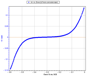
Figure 2: Steady-state curve I vs. E_WE

Note: It is possible to load the different LP_iron_corrosion files with EC-Lab software in the following folder:
C:\Users\…\Documents\EC-Lab\Data\Samples\Corrosion

The Stern relation can be written as followed:

$I = I_\text {corr}\left(\text{exp}\left(\text{ln}10\frac{E-E_\text {corr}}{\beta_\text a}\right)\text{-exp}\left(\text{ln}10\frac{-(E-E_\text {corr})}{\beta_\text c}\right)\right) \tag{1}$

From the graph displaying log |I| vs. E_WE, it is possible to determine the values of I_corr, E_corr, β_a and β_c by a simple analysis.
The Tafel fit, which is a Graph Analysis tool from EC-Lab^®, can determine automatically these values (Fig. 3).

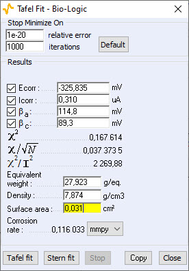
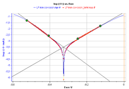
Figure 3: Tafel Fit Analysis.

Note: The corrosion rate can be determined if the user enters the values of the equivalent weight (atomic weight divided by the number of electrons involved in the reaction), the material density and the active surface area.

The expression of the polarization resistance can be defined as:

$$R_\text P = \frac{1}{dI/dE} \tag{2}$$

Which gives, at $E= E_\text {corr}$, using Eq. 1:

$$R_{\text p,E_\text {corr}}=\frac{\beta_\text a \beta_\text c}{I_\text {corr}(\beta_\text a + \beta_\text c)\text{ln}10} \tag{3}$$

and knowing the values of R_p,Ecorr, β_a and β_c, we can figure out the value of I_corr with the following relationship:

$$I_\text{corr}=\frac{\beta_\text a \beta_\text c}{R_{\text p,E_\text {corr}}(\beta_\text a + \beta_\text c)\mathrm{ln}10} \tag{4}$$

The value of R_p,Ecorr can be simply determined by displaying the graph giving E_WE vs. I around the corrosion potential and calculating the slope of the curve.

The R_p fit, which is a graph analysis tool from EC-Lab (cf. Quickstart – Analysis Graph Tools), can automatically calculate the value of R_p. It is also possible to determine the corrosion current I_corr if the values of the Tafel coefficients β_a and β_c are known. The user will just have to type these values in the R_p fit analysis window before the fit (Fig. 4).

Figure 4: R_p fit analysis.

References

- D. Landolt, in : Traité des Matériaux, 12, Presses Polytechniques et Universitaires Romandes (Ed.), (2003).
- J.P. Diard, B. Le Gorrec and C. Montella, in: Cinétique électrochimique, Hermann, (1996) 204.
Revised in 07/2018