

EIS measurements on a RDE Part I: Determination of a diffusion coefficient using the new element Winf Electrochemistry – Application Note 66
Latest updated: July 3, 2026Abstract
In this application note, the BluRev RDE is used along with a potentiostat to perform impedance measurements on a rotating disk electrode. An easy methodology to derive the diffusion constants of the reactive species using the fitting results of the impedance data is also presented. ZFit, the fitting analysis module in EC-Lab®, offers various elements to fit diffusion and convective diffusion impedances (Warburg, $W_\delta$ and $W_\text{inf}$). The element which gives the best approximation of a convective diffusion is the newer element $W_\text{inf}$, for which the goodness of fit is the highest. Another advantage of this element is that it directly gives the diffusion coefficient, without any further calculation as it is the case for the Warburg and $W_\delta$ element.
Introduction
Levich and Koutecký-Levich methods [1] are powerful analysis tools used to obtain kinetic electrochemical parameters such as the diffusion coefficient of a redox species in a given medium and the reaction constant. These analyses require to have potentio-dynamic curves at various rotation speeds.
However, fitting impedance measurements made on a redox reaction occurring at a quiescent or rotating electrode at only one rotation speed also enables the identification of the above-mentioned kinetic parameters.
This first part of the application note will deal with the determination of a diffusion coefficient, while the second part of this note will deal with the determination of the redox reaction kinetic constant. The applications of these analysis tools are extremely wide: electrocatalysis, fuel cells, corrosion, sensors, electroanalytical chemistry, energy storage…
EXPERIMENTAL CONDITIONS
ELECTROLYTE
An equimolar solution of $\text{K}_3\text{Fe(CN)}_6$ and $\text{K}_4\text{Fe(CN)}_6$ with concentrations of 5 mM in 0.1 M KCl is used. The presence of the two species in solution allow us to carry out our experiments around the steady-state equilibrium potential; if there only was one species, the potential taken by the system would be the mixed potential, which is out of equilibrium. In the whole document, it is assumed that the diffusion coefficients of both species are the same. This, and the equimolarity of the two species, allow us to simplify the relationships used to determine diffusion coefficients from impedance data. Further details are given in the Appendix A. The electrochemical redox reaction is the following:
$$[\text{Fe(CN)}_6]^{3-} + \text{e}^- \leftrightarrow [\text{Fe(CN)}_6]^{4-} \tag{1}$$
SET-UP
- Hardware
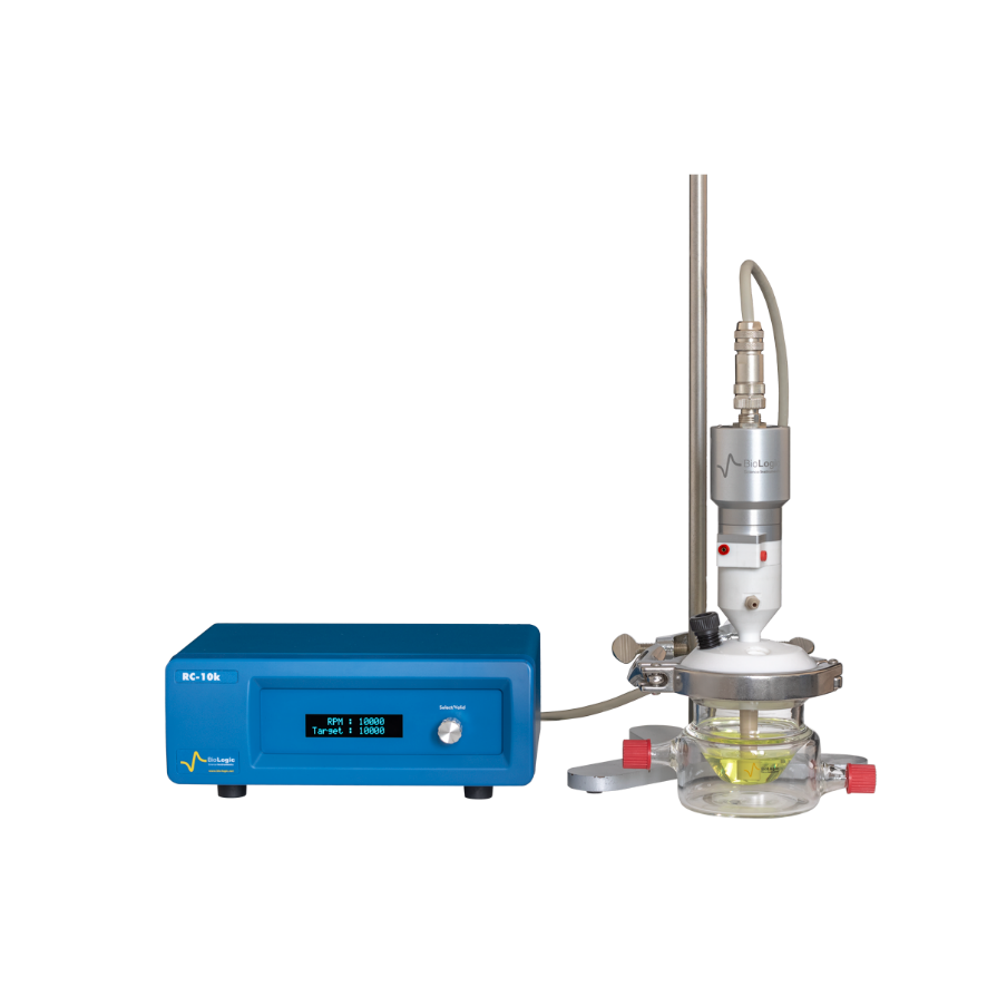
We used a BluRev RDE (094-RC/RDE) and a VMP-3 (any BioLogic potentiostat can be used). The BluRev is composed of a control box called the RC-10k and the RDE itself comprising a motor and a rotating shaft. Electrode tips are then screwed to the end of the shaft. We used a 2 mm Pt disk (094-Pt/2).
To remotely control the rotation speed, one DB9-BNC connector and two BNC-BNC female cables are required, one to control the rotation speed of the electrode and another one to monitor it. They should be connected to the back panel of the RC-10k.
One can also choose to manually control the RC-10k by using the front panel rotary push button.

Figure 1: The BluRev RDE with EL-ELECTRO-1 and Fe(II)/Fe(III) solution.
- Software
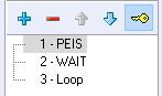
The aim is to perform a series of EIS measurements at different rotation speeds even though one speed only is necessary for the calculations. For the manual control the following linked techniques were used:
PEIS->WAIT->LOOP.
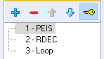
For the external control the following linked techniques were used:
PEIS->RDEC->LOOP
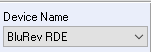
External Devices tab with parameters related to BluRev RDE were also set:
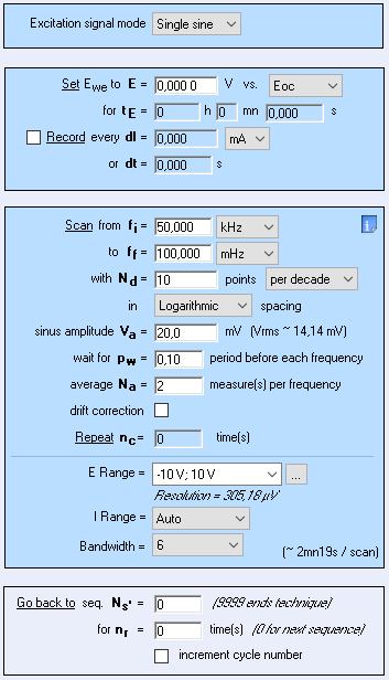
The measurement parameters of the PEIS technique are shown in Fig. 2

Figure 2: Parameters settings of the PEIS technique.
RESULTS
The following results were obtained (Fig. 3):

Figure 3: Nyquist plot of impedance measurements performed using the conditions described in set-up.
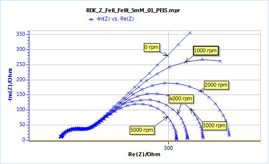
- The higher frequency part of the graphs, which is related to the transfer resistance, (that is to say the resistance related to the actual electron transfer of the redox reaction), does not change with the rotation speed.
- At lower frequencies, the graph at 0 rpm exhibits a semi-infinite diffusion behaviour, that can be fitted with a Warburg element.
- For the graphs obtained with a rotating electrode, the lower parts of the impedance exhibit a diffusion-convection behaviour. As the rotation speed increases, the low frequency limit of the real part of the impedance decreases.
ANALYSIS
All these data can be fitted using ZFit. The determination of the values of the parameters of the equivalent circuit can lead to the determination of physical constants related to the system (i.e., electrolyte + reaction + electrode surface).
ELECTRODE IN QUIESCENT STATE: 0 RPM
One can use the typical Randles equivalent circuit with a Warburg element to account for semi-infinite diffusion as shown in Fig. 4. The fitted curve is shown in Fig. 5.

Figure 4: The Randles circuit
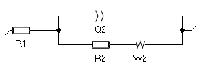

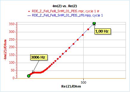
Figure 5: Impedance data obtained on a 2 mm Pt disk electrode in a quiescent state in 5 mM $\text{[Fe(CN)}_6]^{3-}$ and $\text{[Fe(CN)}_6]^{4-}$ and 0.1 M NaCl (red dots) and fitting curve (blue line).
R1 is the electrolyte resistance between the working electrode and the reference electrode; R2 is the transfer resistance; Q2 represents the double-layer capacitance of the electrode/electrolyte interface; W2 is the Warburg impedance associated with the mass transport of the reactive species, here they are only transported by diffusion.
Using Randomize + Simplex minimization procedure, without weighting, fitting the data should give the following results:
R1 = 139.9 Ω; Q2 = 6.057 10-6 F s(a2 – 1); a2 = 0.821; R2 = 79.14 Ω; $\sigma$2 = 896.8 Ω s-1/2; X2 = 97.78 Ω2.
We discuss the meaning of the $\text X^2$ parameter later and how it can be used. One can derive the diffusion constant of the species using the value of the Warburg parameter $\sigma$ and the following relationship [1, Appendix A]:
$$\sigma = \frac{2RT}{F^2 AX^* \sqrt{2D_X}} \tag{2}$$
Hence
$$D_\text X = 2\left(\frac{RT}{(n^2F^2 X^* \sigma A}\right)^2 \tag{3}$$
With:
$D_\text X$ the diffusion coefficient of the species $\text X$ in cm2 s-1, $R$ the perfect gas constant in J mol-1 K-1, $T$ the temperature in K, $F$ the Faraday constant in C mol-1, $\text X^*$ the bulk concentration in mol cm-3 and $A$ the electrode area in cm2.
Using Eq. (3) and the values of the parameters obtained by fitting we have $D_\text X$ = 7.13 10-6 cm2 s-1, which is in agreement with values found in the literature (Tab. I).
Table I: Diffusion coefficient values found in the literature.
| Species | $D_\text X$/10-6 cm2 s-1 | Reference |
|---|---|---|
| $\text{[Fe(CN)}_6]^{3-}$ | 8.96 | [3] |
| 7.6 | [2] | |
| $\text{[Fe(CN)}_6]^{4-}$ | 7.35 | [3] |
| 6.5 | [2] |
With a quiescent electrode, the user needs to know the concentration of the species of interest as well as the electrode area to be able to derive the diffusion coefficient. The species concentration and the area of the reactive electrode can sometimes be unknown.
ROTATING ELECTRODE: 1000 – 5000 RPM
To fit the impedance data, the Randles circuit can also be used but the mass transport element cannot be a Warburg element, as now the mass transport mechanism is not only diffusion but diffusion and convection.
There are two elements available in ZFit to fit low frequency impedance data related to convective diffusion:
- The first one is $W_\delta$. The expression of its impedance is based on the Nernst model approximation: the concentration variations of the species due to the electrochemical reaction only occurs within the diffusion layer. Outside of the diffusion layer (i.e. in the bulk) the concentration is constant. See the Appendix B for the expression of the impedance of $W_\delta$. The corresponding Randles circuit is shown in Fig. 6.

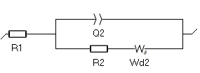
Figure 6: The Randles circuit with the $W_\delta$ element.
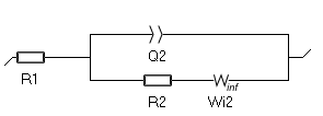
- The second one, available since EC-Lab 11.25, is $W_\text{inf}$. The expression of its impedance is based on the numerical approximation of the analytical description of diffusion-convection at a disk electrode. Its expression is closer to the true situation, where the concentration of the species changes in the entire electrolyte, not only in a confined zone close to the electrode. The corresponding Randles circuit is shown in Fig. 7. See the Appendix C for the expression of the impedance of $W_\text{inf}$.

Figure 7: The Randles circuit with the $W_\text{inf}$ element.
$W_\delta$, the bounded diffusion element
Fitting the data with $W_\delta$, one can derive a time constant $\tau_\text d$, which can be used to obtain the diffusion coefficient of the species of interest, knowing the rotation speed of the electrode and the kinematic viscosity of the fluid.
Assuming that the diffusion constants of both species are the same, the time constant is related to the diffusion coefficient by the following relationship:
$$\tau_d = k_{\text L}^2 D_{\text X}^{-1/3} \nu^{1/3} \Omega^{-1} \tag{4}$$
Where $k_\text L$ is a constant equal to 1.611, $\nu$ is the kinematic viscosity of the electrolyte in cm2 s-1, $D_\text X$ the diffusion coefficient in cm2 s-1 and Ω is the rotation speed in rad s-1.
Two approaches can be chosen: either one decides to calculate the diffusion coefficient from the results obtained at one single rotation speed or one can choose to calculate the time constant at each rotation speed and to plot it as a function of the inverse of the rotation speed, in which case the slope is expressed as:
$$p=k_{\text L}^2 D_{\text X}^{-1/3} \nu^{1/3} \tag{5}$$
And hence
$$D_{\text X} = k_{\text L}^6 \nu p^{-3} \tag{6}$$
Obtaining the diffusion coefficient using this method gives a more “robust” number as it averaged over five values. Figure 8a shows an example of an experimental curve fitted using the equivalent circuit shown in Fig. 6, as well as a close-up in Fig. 8b.


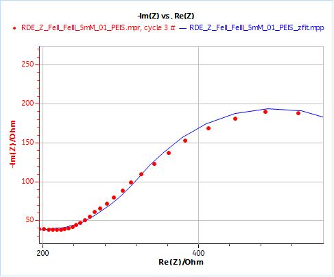
Figure 8: a) Nyquist plot of impedance measurements performed using the conditions described in I-2, at a rotation speed of 2000 rpm (red dots) and the fitting curve using equivalent circuit shown in Fig. 5 (blue line); b) Close-up ; c) Residuals between experimental points and fitting data in %.
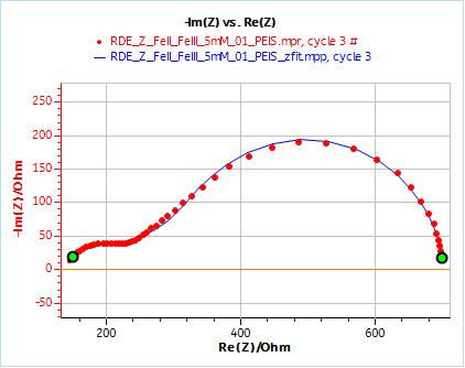
The results corresponding to Fig. 8 are R1 = 129.8 Ω; Q2 = 25.95 10-6 F sa2 – 1; a2 = 0.65; R2 = 115.3 Ω; Rd2 = 460.2 Ω; td2 = 0.148 s; X2 = 588.4 Ω2.
Fitting the data at all rotation speeds, extracting the parameter $\tau_\text d$ (td in ZFit) and plotting it against the inverse of the rotation speed gives the curve shown in Fig. 9.

Figure 9: Time constants $\tau_\text d$ vs. $\Omega^{-1}$ the inverse of the rotation speeds. The slope can be used to determine the diffusion coefficient.
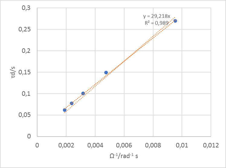
Using the slope of this curve p (here 29.21 rad) in Eq. (6), with $\nu$ = 10-2 cm2 s-1, one gets $D_\text X$ = 7.01 10-6 cm2 s-1.
$W_\text{inf}$ the analytical approximation element
This element represents a better approximation of a redox reaction limited by convective diffusion. Furthermore, the expression of its impedance allows to use as a parameter of the fit the diffusion coefficient of the reactive species, assuming in our case that the diffusion coefficients of both species are the same.
As an example, Figs. 10 and 11 show the results obtained by fitting the impedance data at 2000 rpm. One just needs to enter the rotation rate in rpm and the kinematic viscosity in cm2 s-1. Similarly, one just needs to carry out an impedance measurement at one single rotation speed to directly obtain the diffusion coefficient of the species.


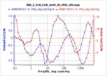
Figure 10: Nyquist plot of impedance measurements performed using the conditions described in I-2, at a rotation speed of 2000 rpm (red dots) and the fitting curve using equivalent circuit shown in Fig. 7 (blue line); b) Close-up ; c) Residuals between experimental points and fitting data in %.
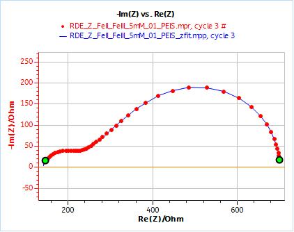
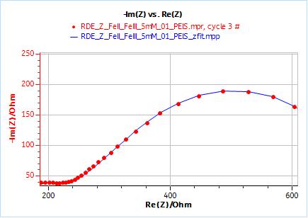
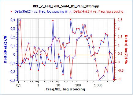

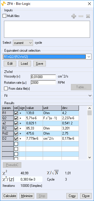
Figure 11: ZFit analysis window showing the fitting results obtained with a Randles circuit and $W_\text{inf}$ element on data obtained at 2000 rpm. The obtained diffusion coefficient is equal to 7.78 10-6 cm2 s-1.
One can also try to fit data obtained at several speeds to test the robustness of the value and choose to take an average value, as shown in the table below:
Table II: Diffusion coefficients values calculated at different rotation rates using ZFit and $W_\text{inf}$ element in a Randles circuit (Fig. 7).
| $\Omega$/103 rpm | 1 | 2 | 3 | 4 | 5 |
|---|---|---|---|---|---|
| $D_\text X$/ 10-6 cm2 s-1 | 8.32 | 7.78 | 7.95 | 7.90 | 8.07 |
The average value is 8.00 10-6 cm2 s-1, which is larger than the two values obtained before-hand with $W$ and $W_\delta$ elements.
DISCUSSION
We have seen that there are three different ways to obtain the diffusion coefficients. How can we decide which way is the right one?
As previously stated, fitting with $W_\text{inf}$ allows a direct determination of the diffusion coefficient knowing the electrode rotation speed and the kinematic viscosity of the electrolyte. Using the Warburg element on a quiescent electrode to obtain the diffusion coefficient requires to know the species concentration and the area at which the reaction occurs.
Furthermore, one can compare the correctness or relevance of each element to fit the data. It can be done qualitatively by comparing the experimental points and the fitted curve: one can see in Fig. 8b that the fitting curve does not go through the data points. It goes below and above the data points. In Fig 9b, obtained using $W_\text{inf}$, the fitting curve goes through all data points.
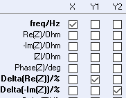
This qualitative observation is confirmed by the residual plots shown in Figs. 8c and 9c. There residuals are the difference in percentage of the fitting data and the experimental points. It is readily accessible in EC-Lab® using the variables selector:

In the case of $W_\delta$, the residuals are in the range of ±1.5 % and +15/-5 %, for Re(Z) and Im(Z) respectively.
In the case of $W_\text{inf}$, the residuals are in the range of ±0.4 % and +2.5/-1 %, for Re(Z) and Im(Z) respectively.
Finally, the $\chi^2$ factor, which is an indicator of the goodness of the fit, can be used to compare the methods. The formula is the following:
$$\chi^2=\Sigma_{i=1}^N|Z_i (f_i)-Z(f_i)|^2 \tag{7}$$
with $Z_i$ the measured impedance and $Z(f_i)$ the value of the impedance calculated at a frequency $f_i$ for a defined set of parameter values and N the number of points.
Table III shows the values of $\chi^2$ for data fitted with the various elements.
Table III: $\chi^2$ comparisons for $W_\delta$ and $W_\text{inf}$.
| Element | $W_\delta$ | $W_\text{inf}$ |
| Rotation speed/rpm | 2000 | 2000 |
| $\chi^2$/$\Omega^2$ | 588.4 | 48.99 |
According to $\chi^2$, the best fit is obtained using $W_\text{inf}$.
SUMMARY
Table IV: Requirements for the determination of the diffusion coefficient.
| $W$ | $W_\delta$ | $W_\text{inf}$ | |
| No RDE | Post-fit calculation, surface, concentration | N/A | N/A |
| RDE | N/A | Post-fit calculation | None |
Conclusion
In this application note, we have seen how the BluRev RDE can be used along with a potentiostat to perform impedance measurements on a rotating disk electrode. More importantly, we have shown the methodology to derive the diffusion constants of the reactive species using the fitting results of the impedance data. ZFit, the fitting analysis module in EC-Lab®, offers various elements to fit diffusion and convective diffusion impedances (Warburg, $W_\delta$ and $W_\text{inf}$). The element which gives the best approximation of a convective diffusion is the element $W_\text{inf}$, for which the goodness of fit is the highest. Another advantage of this element is that it directly gives the diffusion coefficient, without any further calculation as it is the case for the Warburg and $W_\delta$ element. $W_\delta$ could be used for specific cases such as thin layer electrochemistry where the electrolyte layer is as thick as the diffusion layer or ion exchange membranes.
APPENDIX
A – Expression of the concentration impedance of dissolved electroactive species at a quiescent electrode
The total concentration impedance is the sum of the impedance of each redox species O and R. We have [2]:
$$Z_{\text W} (\omega)=Z_\text O (\omega)+Z_\text R (\omega)=\frac{\sqrt2 \sigma}{\sqrt{j \omega}} \tag{8}$$
With
$$\sigma = \frac{RT}{F^2 A\sqrt{2}}\left( \frac{1}{\sqrt{D_\text O}C^*_\text O} + \frac{1}{\sqrt{D_\text R}C^*_\text R} \right) \tag{9}$$
In the case where both species are at the same bulk concentration we have:
$$\sigma = \frac{RT}{F^2 A\sqrt{2} C_{\text X}^*}\left( \frac{1}{\sqrt{D_\text O}} + \frac{1}{\sqrt{D_\text R}} \right) \tag{10}$$
Assuming that both diffusion coefficients are equal to $D_\text X$, we obtain Eq. (2).
B – Expression of the concentration impedance of dissolved electroactive species at a rotating electrode using the Nernst approximation [4-8]
Considering one diffusing species X, the expression of the impedance of the $W_\delta$ element is:
$$Z_{\text W_{\delta}} (\omega) = R_\text d \frac{\text{tanh}\sqrt{\tau_\text d j \omega}}{\sqrt{\tau_\text d j \omega}} \tag{11}$$
With
$$\tau_\text d = \frac{\delta^2_\text X}{D_\text X} \tag{12}$$
C – Expression of the concentration impedance of dissolved electroactive species at a rotating electrode using the analytical approximation [9,10]
This analytical approximation is an improvement of previous work [11]
$$Z_{\text W_\text {inf}}(\omega) = R_\text d \frac{\sqrt{\gamma^2 + \tau_\text d j \omega}}{\gamma + \tau_\text d j \omega} \tag{13}$$
With
$$\gamma = \frac{1.9930-1.6319 \, \text{Sc}^{-1/3}}{1-0.7248 \, \text{Sc}^{-1/3}} \tag{14}$$
$$\text{Sc} = \frac{\nu}{D_\text X} \tag{15}$$
$$\tau_\text d = \frac{1.61173^2}{\Omega} \, \text{Sc}^{1/3} (1+0.2980 \, \text{Sc}^{-1/3}+0.14514 \, \text{Sc}^{-2/3} + 0.07020 \, \text{Sc}^{-1})^2 \tag{16}$$
References
- Application Note #56 “Electrochemical reaction kinetics measurement: the Levich and Koutecký-Levich analysis tools”
- A. J. Bard, W. Faulkner, in: Electrochemical Methods, Fundamentals and Applications,2nd Ed., Wiley, New York (2001) 381.
- D. R. Lide, H. V. Kehiaian, in: CRC handbook of thermophysical and thermochemical data, CRC Press, Inc., Boca Raton, (1994)
- J. Llopis, and F. Colom, in Proceedings of the Eighth Meeting of the C.I.T.C.E., C.I.T.C.E., Butterworths, London (1958) 144.
- J. H. Sluyters, PhD thesis, Utrecht, 1956.
- A. B. Yzermans, PhD thesis, Utrecht, 1965.
- P. Drossbach and J. Schultz J. Electrochim. Acta 11 (1964) 1391.
- D. Schuhmann, Compt. rend. 262 (1966), 1125.
- R. Michel and C. Montella, J. Electroanal. Chem. 736, (2015) 139.
- J.-P. Diard, and C. Montella, J. Electroanal. Chem. 742, (2015) 37.
- C. Deslouis, C. Gabrielli, and B. Tribollet, J. Electrochem. Soc. 130, 10 (1983) 2044.
Last Updated on 26/02/19.


