

Levich and Koutecký-Levich analysis tools: Electrochemical reaction kinetics measurement Kinetics – Application Note 56
Latest updated: January 31, 2024Abstract This note describes these analysis tools that can be used to analyse data obtained with a Rotating Disk Electrode (RDE). Kinetic information such as diffusion coefficient, symmetry factor and standard constant of redox reactions can be determined.
Introduction
Since EC-Lab v11.00, the Levich and Koutecký-Levich analysis tools are available. This note aims to describe what is performed during this analysis and which information can be obtained.
The Rotating Disk Electrode (RDE) allows the user to control the velocity of the fluid. The steady-state mass transport conditions of the species involved in the redox reactions are therefor known [1,2]. The renewal of the solution at a disk electrode occurs thanks to an ascending movement of the solution perpendicularly to the electrode. The fluid is then ejected on the outside of the disk electrode (Fig. 1).

Figure 1: Fluid movement at a uniformly rotating disk electrode. Vx is the axial velocity of the fluid

The control of the steady-state hydrodynamics of the fluids results in solving the kinetic reactions of the redox reactions. Several relationships can also be deduced that lead to the determination of kinetic factors of the considered species and redox reactions: The Levich relationship can be used to determine the diffusion coefficient of the electroactive species and the Koutecký-Levich analysis can lead to the standard constant of the reaction as well as the symmetry factor α.
ROTATING DISK ELECTRODE EXPERIMENT: LEVICH CRITERION
AIM AND PRINCIPLES
The aim of this experiment is to determine the diffusion coefficient or the concentration of the redox species. Whatever the value of the rate constant of the electronic transfer of the studied reaction k°, there is always an overpotential for which the reaction rate will be limited by mass transfer, whether it is diffusion, as it is the case at an Ultra Micro Electrode (UME) or diffusion and convection, as it is the case for an RDE.
At an RDE submitted to a large overpotential, the current density (i=I/A, where A is the area of the electrode) is expressed as
$$i_\text{dR}=0.620nFR^{\text{bulk}}D_\text R^{2/3}\nu^{-1/6}\omega^{1/2} \tag{1}$$
in the case of the oxidation of the species R and
$$i_\text{dO}=-0.620nFO^{\text{bulk}}D_\text O^{2/3}\nu^{-1/6}\omega^{1/2} \tag{2}$$
in the case of the reduction of the species O, where idR and idO are the mass transport limited current densities for an oxidation reaction and a reduction reaction, respectively; n the number of electrons involved in the reaction, F the Faraday constant (96500 C/mol), Rbulk and Obulk the bulk concentration of the species R and O, respectively in mol/cm3, DR and DO the diffusion coefficients of R and O, respectively in cm²/s and ω the rotation rate in rad/s.
Plotting the value of the mass transport limitation current as a function of the square root of the rotation speed, the graph should be a straight line (the Levich plot), with a slope that can be named the Levich slope.
The values of this slope for the oxidation is:
$$p_\text{La}=0.620nFR^{\text{bulk}}D_\text R^{2/3}\nu^{-1/6} \tag{3}$$
And for the reduction:
$$p_\text{Lc}=-0.620nFO^{\text{bulk}}D_\text O^{2/3}\nu^{-1/6} \tag{4}$$
Knowing the concentration of the species and the viscosity of the electrolyte, the diffusion constants of the redox species can be obtained.
EXPERIMENT
The electrolyte used contains K3[Fe(CN)6] and K4[Fe(CN)6] in an equimolar concentration of 0.005 mol/L of and KCl at a concentration of 0.1 mol/L. Let us consider that the temperature of the electrolyte is 20 °C and that its kinematic viscosity is 10-2 cm²/s. The electrode is a 2 mm diameter Pt disk (094- Pt/2). The reaction occurring at the disk is:
$$[\text{Fe(CN)}_6]^{3-} + \text e^- \longleftrightarrow [\text{Fe(CN)}_6]^{-4} \tag{5}$$
The BluRev RDE was used for this experiment (Fig. 2). 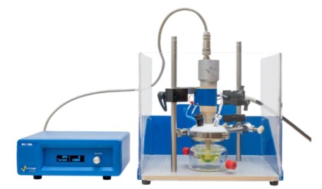 Figure 2: The BluRev RDE with EL-BLUREV, the BluRev enclosure (094-ENCL) and FeII/FeIII solution. Connect only one channel of the potentiostat to the cell using standard connection. The “Levich plot” experiment will load a series of techniques necessary to perform the Levich experiment (Fig. 3).
  Figure 3: The “Levich plot” experiment. The following parameters should be entered in the CV technique (Fig. 4).
  Figure 4: Settings to be entered in the CV technique. The following rotation rates were entered in the RDEC technique: 500, 1000, 2000, 3000, 4000, 5000 RPM. The OCV should be around 0.1 -0.3 V/Ag/AgCl.
The obtained results are shown in Fig. 5.
A hysteresis can be seen at the lower rotation rates, which shows that the experiment is not in the steady-state conditions, probably due to a scanning rate that is too fast. As the rotation speed increases, the conditions tend to be steady-state, for the same scan rate.  Figure 5: Results of the Levich plot experiment for FeII/FeIII oxidation/reduction. The current plateaus occur at potentials for which the reaction is limited by mass transfer.
ANALYSIS
Open the Levich Analysis window (Fig. 6):  Figure 6: The Levich Analysis window Enter the parameters shown in Fig. 6 for the viscosity, the surface of the electrode, and the concentration of FeIII (the diffusion coefficient will be calculated by the analysis). The equation of the Levich current shown in Fig. 7 is the same as the Eqs. (1) and (2) apart from the coefficient, which is different because the equation above is written for a rotation speed in rotation per minute (RPM) as is used in ECLab. The diffusion coefficient is the sought after value so it must be selected. Click on “Calculate”, the Levich plot should appear: the experimental points and the least square regression plot (Fig. 8).
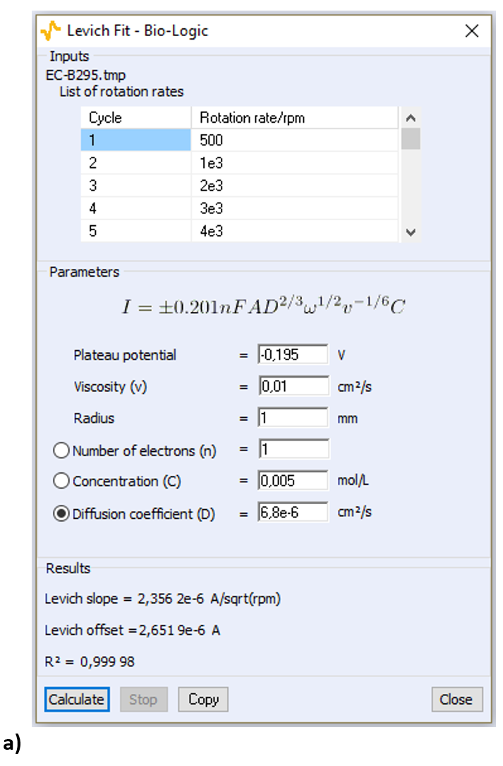
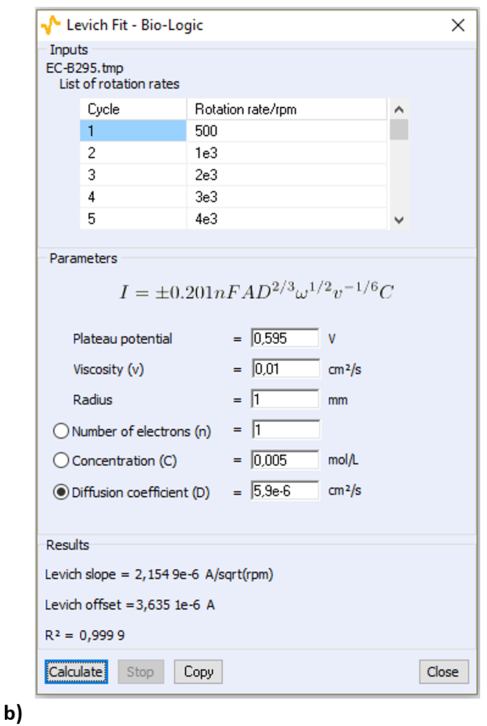
Figure 7: The Levich analysis window a) for the cathodic part and b) the anodic part of the curves shown in Fig. 5.
 Figure 8: The Levich plot showing the mass transfer limited current at a potential of 0.05 V for all the rotations vs. the square root of the rotation rate
The calculated value of D[Fe(CN)6]3− is 6.8 10-6 cm²/s. The same analysis can be performed on the anodic part of the curves, for example by choosing a plateau potential of 0.595 V. The calculated value of D[Fe(CN)6]4− is 5.9 10-6 cm²/s. The same results can be used to determine the concentration of the species in solution knowing its diffusion coefficient. In the analysis window (Fig. 7) the concentration must be selected as the parameter to be calculated.
The same results can be analysed using the Koutecký-Levich extrapolation to determine the reaction standard constant as well as the symmetry factor α.
ROTATING DISK ELECTRODE EXPERIMENT: KOUTECKÝ-LEVICH EXTRAPOLATION
AIM AND METHOD
The aim of the Koutecký-Levich extrapolation is to determine for various potentials En the electron transfer current it. It can also be used to determine the symmetry factor α, (αr for a reduction reaction and αo for an oxidation reaction) as well as the standard constant of the reaction k°, knowing the standard potential E° of the reaction (5).
The method consists in:
- Plotting the inverse of the current or current density as a function of the inverse square root of the rotation rate expressed in rpm for various potentials En.
- Extrapolating the obtained line to 0 gives the current for infinite rotation speed (Ω−1⁄2⟶ 0 ⇔ Ω ⟶ ∞), that is to say the electron transfer current Itfor various potentials En.
- Plotting log|It| as a function of En (Tafel representation) to obtain the symmetry factor α using the slope and the standard constant of the reaction using the current at the standard potential.
The expression of the Tafel slope for a cathodic reaction is:
$$p_\text{Tc} = \frac{\alpha_\text r nF}{RT \; \text{ln 10}} \tag{6}$$
With αrthe symmetry factor of the reduction reaction (αr= 1 − αo).
The expression of the current at the standard potential E°O/R is:
$$\text{log}|I_\text t|_{E^°_\text{O/R}} = \text{log}(nFk°O^{\text{bulk}}) \tag{7}$$
ANALYSIS
Using the same data as for the Levich analysis, open the Koutecký-Levich analysis tool (Fig. 10). In the analysis parameters window in Fig. 9 enter the Parameters as shown and click on “Calculate”.  Figure 9: How to start the Koutecký-Levich analysis. Two windows will then open:
For each chosen potential, 1/I vs. ω-1/2 (Fig. 10).
 Figure 10: The Koutecký-Levich extrapolation plot
The Tafel plot log|It| vs. E, the values It having been obtained by extrapolating the 1/I vs. ω-1/2→ 0 for each potential step (Fig. 11).
 Figure 11: The Koutecký-Levich reconstructed Tafel plot.
The Koutecký-Levich analysis window will show the results of the analysis. Figure 12a and 12b shows the results for the cathodic and anodic part, respectively, of the curve shown in Fig. 5. Both calculated standard constants of the reaction are similar. The calculation will be more accurate if the selected potentials lead to a straight Tafel plot (in log representation). Larger values of k° could be obtained by better cleaning the RDE for instance.
It must be noted that the determination of the electronic transfer kinetic parameters using the Koutecký-Levich method is practically possible for values of k°≤ several 10-2 cm²/s, i.e. sluggish kinetics.
For higher values, the extrapolated values of It-1 are too close to 0 and the uncertainties on their inverse values are too large to allow a good k° determination.
It can be seen in Fig. 10: all lines should be parallel. In this intermediate case, all the lines are secant but It-1 are not too close to 0. For more information please see references [1,2,4,5].
Some people misuse the Koutecký-Levich analysis and try to determine the number of electrons. This last part will explain why people should refrain from doing so. 
 Figure 12: The Koutecký-Levich analysis window for a) the cathodic part and b) the anodic part of the curves shown in Fig. 5.
DETERMINATION OF THE NUMBER OF ELECTRONS BY THE KOUTECKÝ-LEVICH METHOD
In the case of a “quasi-reversible” (or neither reversible nor irreversible) reaction, the slope of the Koutecký-Levich extrapolation plot shown in Fig. 10 is expressed as [1,2]:
$$p_\text{KL}=\frac{1.611\upsilon^{1/6}(D_\text R^{-2/3}\text{exp}\xi+D_O^{-2/3})}{(nF(R^{\mathrm{bulk}}\mathrm{exp}\xi-O^{\mathrm{bulk}})} \tag{8}$$
With ξ = nf(E − E°O/R) and f = F/(RT). The slope depends on the electrode potential. In the case of an irreversible reaction, the slope of Koutecký-Levich extrapolation plots is expressed as:
$$p_\text{KL}=\frac{1.611\upsilon^{1/6}}{(nFD_\text O^{2/3}O^{\text{bulk}})} \tag{9}$$
In this case, the slope does not depend on the electrode potential. For an irreversible reaction, the Koutecký-Levich extrapolation plots shown in Figure 10 would all be parallel and independent from the electrode potential. In this case only, Eq. (9) could be used to determine the number of electrons involved in the reaction. But in this case, it is equivalent to the Levich analysis. One can see that Eq. (9) and Eq. (4) are equivalent.
Conclusion
The “Levich plot” technique as well as the Levich and Koutecký-Levich analyses were presented. The Levich analysis allows the user to determine the diffusion constant of a reactive species and the Koutecký-Levich extrapolation method allows for sluggish kinetics to determine the kinetic parameters (k° and the symmetry factor α) of the electronic transfer for the considered reaction. The Koutecký-Levich analysis should be used to determine the number of electrons involved in the reaction only if it is irreversible.
Data files can be found in: C:\Users\xxx\Documents\ECLab\Data\Samples\Fundamental Electrochemistry\ AN56_CV
Latest modification on 8/2020
References
1) J.-P. Diard, B. Le Gorrec, C. Montella, Cinétique électrochimique, Hermann, Paris, (1996) 120-129.
2) A. J. Bard, L. R. Faulkner, Electrochemical methods, Fundamentals and Applications, 2nd ed., Wiley, New York, (2001) 335.
3) Technical Note#21 “External device control and recording”
4) F. J. Vidal-Iglesias, J. Solla-Gullón, V. Montiel, A. Aldaz, Electrochem. Com. 15 (2012) 42.
5) J. Koutecký, B.G. Levich, Zhurnal Fizicheskoi Khimii USSR 32 (1958) 1565.


