Post-treatment and optimization of area scan experimentsScanning Probes – Application Note 4

Introduction.

It may be the case that the time taken to setup and closely examine a sample can in-itself, be off- putting to experimentation; after all, everyone works to deadlines. One method that can help alleviate the time investment is the ability to either enhance data or find data within a noisy signal. With this ability, quicker and coarser measurements can be made.
This tech-note demonstrates the use of four data processing methods that are effectively instantaneous on today’s PCs, and are applied to data that was specifically set to acquire as fast (and noisy) as possible so that the overall time to find a result was reduced.
The case demonstrated here is an SKP sample that is not particularly levelled and an instrument setup that has not been optimised to extract meaningful data. The result, as might be expected, is very poor. The data are then processed to reveal a small (few microns) indentation at the point near the centre of the scan. Once this is emphasised, closer inspection is made for comparison purposes.

A fast CHM measurement.

For the purposes of demonstration, a standard SKP sample was mounted in a TriCell™ base with only the briefest attempt at levelling the sample. An SKP probe was then brought to 160 µm of the surface (typically, this would be closer to 100 µm) and a CHM experiment quickly configured.
In this case, the setup was to scan the surface at 2 mm/s with no delay made in any sample or line and no conditioning time set. The electronics was set to allow all signal and noise through to the acquisition system with as little filtering as possible. In total, 51 x 51 points were imaged over 5 mm2 (total, 2601 points) and was completed in 4 min 48 s. The result is shown in Fig. 1.

Figure 1: Left: Basic “fast” test result over 25 mm2. Right: Right-Click Analysis menu.

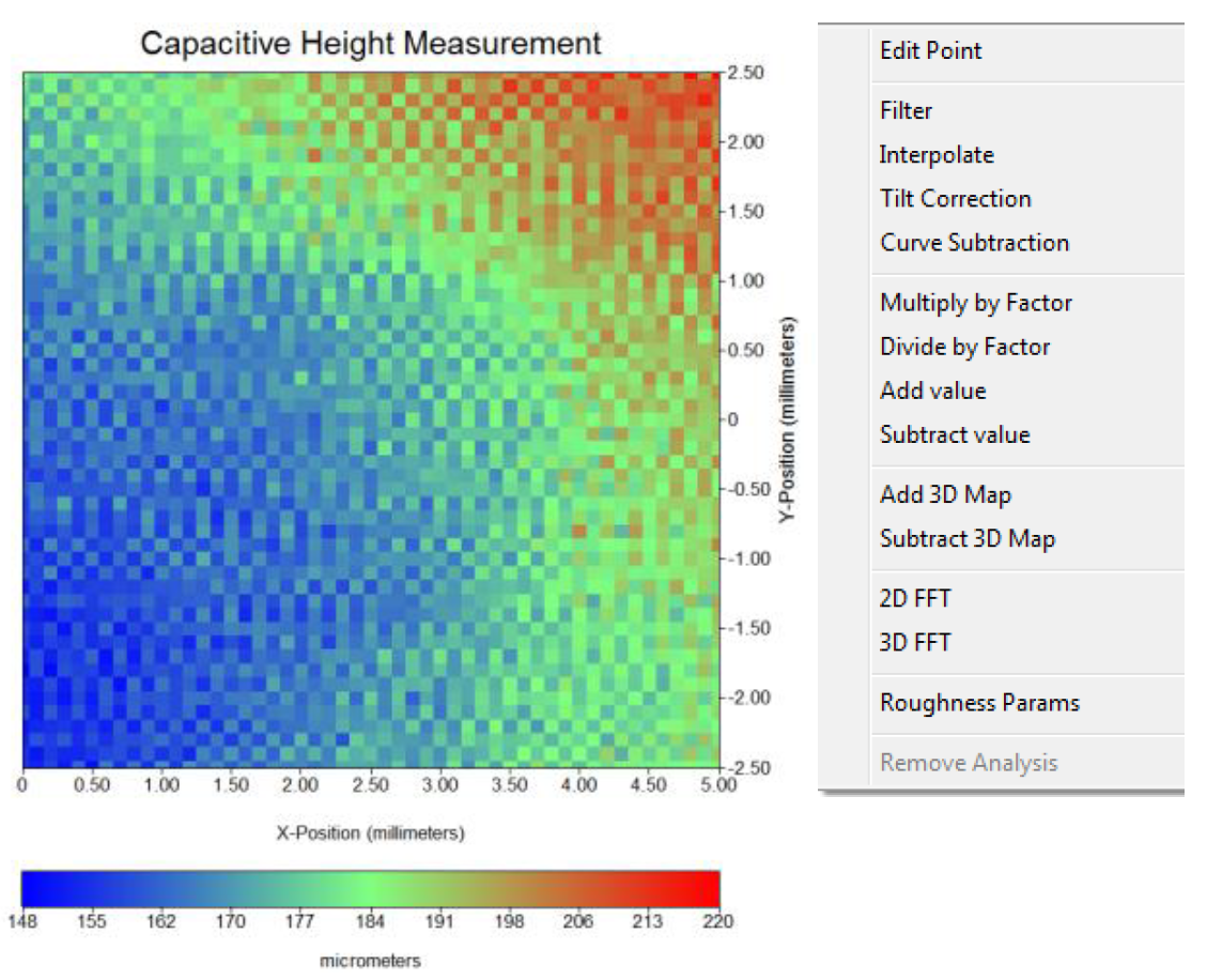
As can be seen from the above, there is little to suggest a region that has any point of interest. However, by applying the analysis functions “Tilt Correction”, “Filter”, “Curve Subtraction” and “Interpolate”, the results are immediately apparent:

Figure 2: Application of analysis functions.

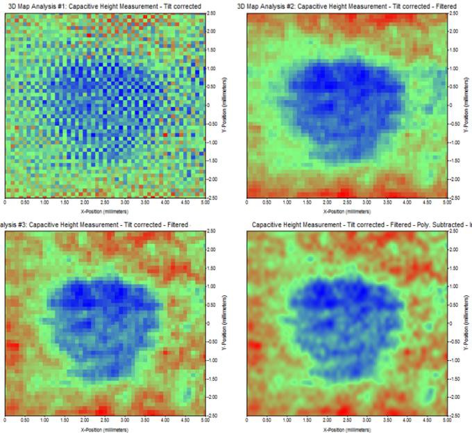
In Fig. 2, the top left image is produced by the “Tilt-Correction” analysis option. This option finds the plane of best-fit from the data selected by the user. This plane is then found and subtracted from the data.
Once the data are effectively levelled the next image (Figure 2, top right) is produced by filtering the data. This is achieved by selecting the “Filter” analysis option. This option “Fourier-filters” the data. The user is then required to input the filter type (here, Low Pass), a cut-off frequency and a roll-off. Here, the spatial cut-off frequency was determined by inspection of the data and the filter chosen to have a cut-off of around 4000 m-1. The filter order was set to 5 for a fast roll-off and the process was then allowed to complete.
As the result of the Fourier filter looked rounded at the top and bottom edges, the “Curve Subtraction” analysis option was chosen. Here a polynomial of best fit is made to a selection of data chosen by the user. This is done in a single axis, here the ‘Y’ axis, and a Quartic polynomial chosen to help remove the upturned data edges. The result is shown in Fig. 2, bottom left.
Finally, the Curve-Subtracted data was interpolated from 51 x 51 points up to 201 x 201 points and the result is shown in Fig. 2, bottom right, and also in Fig. 3 on the left.
For comparison, the sample was then levelled and the system set up more appropriately. A comparison of both results side-by-side can be seen in Fig. 3.

Figure 3: Left: Noisy fast-scan data, post processed. Right: slower, more considered approach to acquiring data.

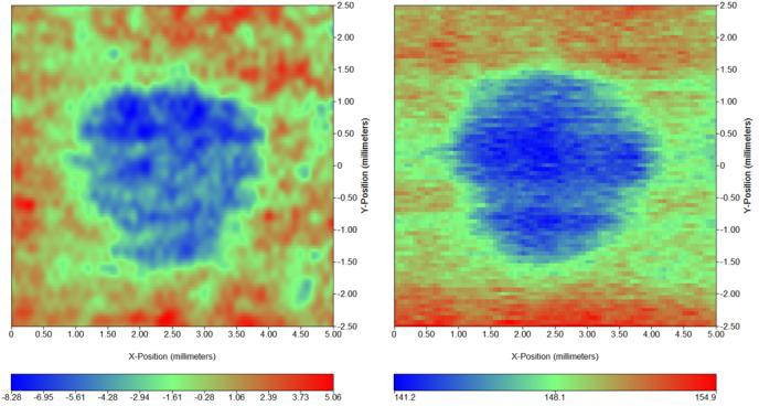
On the left side of Fig.3, the data are the same as shown if Fig. 2 bottom right: data were noisy and obtained and a unlevelled sample. The time taken to acquire them was 4 min 48 s. On the right side, the sample was levelled and data were acquired at a much slower rate. The total time taken was 21 min 52 s. The sweep scan was slower (400 µm/s instead of 2000 µm/s) and the step size was smaller (62.5 µm instead of 100 µm).

Conclusions.

This application note showed the range of post- treatment analysis tool that are available in the M370 and M470 software and can be used to extract meaningful data. These tools are the following : tilt correction, filtering, curve substraction and interpolation. In spite of the abilities of these powerful tools, the user must bear in mind that the best way to obtain meaningful data and reduce noise is to suitably configure the experiments. The drawback of this is that the measurement will be longer.