

IMVS investigation on photovoltaic cell (IMVS) Photovoltaics – Application Note 30
Latest updated: January 31, 2024Abstract
This Application Note describes the experimental setup, data collection and data processing methods for measuring intensity-modulated photovoltage spectra of photovoltaic cells. An LED light source is powered by the potentiostat channel while the photovoltage of the PV cell is measured, simultaneously. The Staircase Galvano-EIS (SGEIS) Technique is used.
Introduction
To carry out electrochemical investigations, several techniques are available. Among these techniques, Electrochemical Impedance Spectroscopy (EIS) technique is used intensively. This technique leads to kinetic characterizations. In EIS investigations, sinusoidal excitations are carried out by current or potential oscillations, respectively named galvano- or potentio-EIS. Depending on the system being studied, the use of nonelectrical modulation can be useful [1-2]. Consequently, such techniques are no longer called EIS but more generally referred to as transmittance spectroscopy.
In the context of the photovoltaic cell (PV) characterization, it could be useful to measure the modulation of photovoltage or photo-current in response to the modulation of incident light intensity [3-5]. The names of these photo-transmittance techniques are Intensity Modulated photoVoltage Spectroscopy (IMVS) and Intensity Modulated Photocurrent Spectroscopy (IMPS).
Principle of IMVS and IMPS is summarized in Fig. 1.
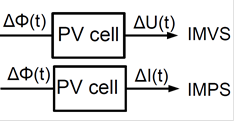
Figure 1: IMVS and IMPS principle; where ΔΦ is the variation of the photon flux, ΔI is the variation of the cell current and ΔU is the variation of the cell voltage.
The corresponding transfer functions HIMVS and HIMPS of the IMVS and IMPS techniques are respectively defined by the following relationship (where ℒ is the Laplace Transform and s is the Laplace variable):
$$H^{(\text{s})}_{\text{IMVS}}=\frac{\text{L} \Delta U(t)}{\text{L} \Delta \Phi (t)}$$
$$H^{(\text{s})}_{\text{IMpS}}=\frac{\text{L} \Delta I(t)}{\text{L} \Delta \Phi (t)}$$
This note is focused on IMVS technique. First of all, experimental information such as cell connection (only one channel is required) and technique settings will be presented in this note. We will discuss data analysis in the last section.
N.B.: All settings and raw data files presented hereafter are available in the Data Sample folder of EC-Lab® Software with the following name: technique_IMVS.mpr.
Set-up description
The variation of the photon flux is performed with a white LED (blue LED + yellow phosphorus). The main LED characteristics are:
- viewing angle of the LED is 15°,
- wavelength characteristics are given by the following figure:
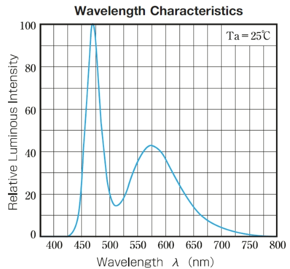
Figure 2: Wavelength characteristics of the white LED.
Taking into account the LED angle and the distance PV cell/LED (9 cm), the light power is given in Tab.I:
Table I: DC current and corresponding light power.
| DC current/mA | Light power/W·m-2 |
|---|---|
| 5.0 | 0.500 |
| 5.0 | 0.500 |
| 7.5 | 0.750 |
| 10.0 | 1.000 |
| 12.5 | 1.250 |
| 15.0 | 1.500 |
| 17.5 | 1.750 |
| 20 | 2.000 |
| 22.5 | 2.250 |
| 25.0 | 2.500 |
| 27.5 | 2.750 |
| 30.0 | 3.000 |
The AC and DC currents were applied by a SP-300 potentiostat/galvanostat instrument. In order to manage the AC/DC current, the CA1 and CA2 leads controlling the current are connected to the LED. The voltage measurements at the PV cell were carried out with the leads Ref1 and Ref2. Connection details are described in the Fig. 3:
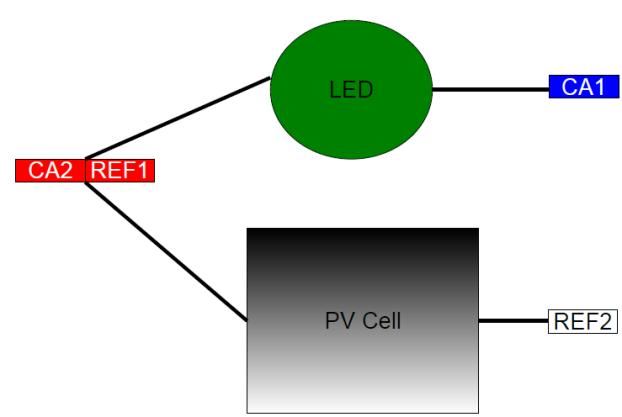
Figure 3: LED, potentiostat/galvanostat/EIS, photovoltaic cell connection.
It is important to note that with this specific configuration, only one channel is required to perform IMVS investigations (control the LED light and measure the PV cell voltage).
Note that all the experiment can be carried out with any galvanostat/potentiostat instruments with EIS ability from BioLogic Science Instruments.
IMVS measurements
LED characterization
Before starting IMVS investigations, the linearity of the relationship between the applied current to the LED and the light emitted by the LED is investigated.
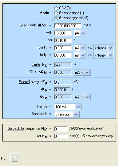
Figure 4: Modular Galvano dynamic technique setting.
A current scan is performed with the Modular Galvano dynamic technique between 0 and 30 mA. Then, the intensity of the emitted light is measured by a photomultiplier, PMS-250 (BioLogic Science Instruments) controlled by Bio-Kine software.
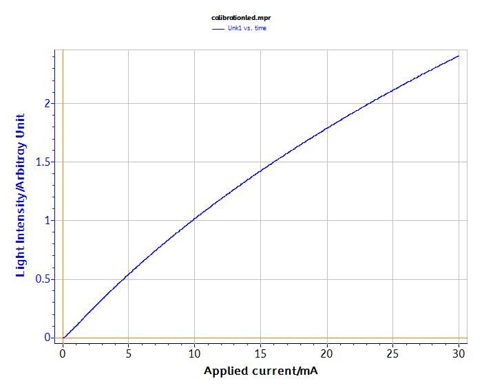
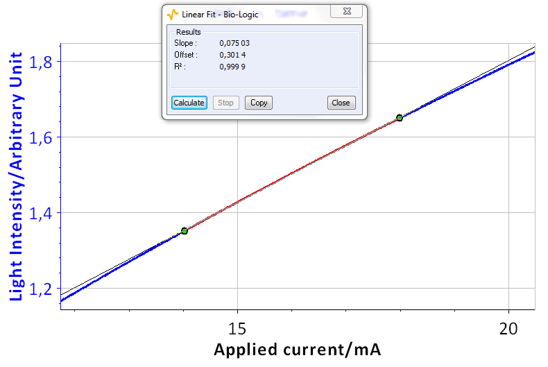
The resulting curve shows that the relationship is not linear over all the range of current i.e. 0 to 30 mA (Fig. 5 top), but linear within a sharper range, for instance a range of 4 mA between 14 and 18 mA (Fig. 5 bottom). As IMVS is performed with small current modulation, the relationship between current and emitted light intensity is considered as linear (no correction parameter is needed). Consequently, it is assumed that the variation of the photon flux (ΔΦ) is equal to variation of the applied current to the LED.


Figure 5: Relationship between light intensity and applied current. Top: between 0 to 30 mA, bottom: zoom between 14 and 18 mA.
IMVS characterization
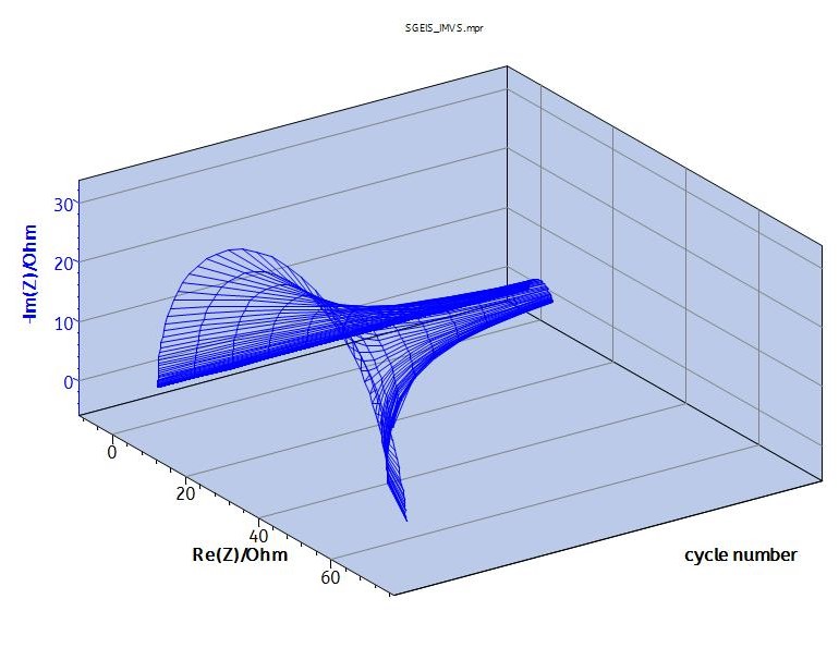
The dedicated technique to perform IMVS is the Staircase Galvano-EIS (SGEIS). Indeed, this technique allows users to apply successive DC levels and superimpose to this DC level an AC current (Fig. 6).
In our case, a scan with 10 steps of DC current is applied from 5 to 30 mA, respectively Ii and If in Fig. 6 and 7. This corresponds to the DC component of the superimposed. A modulation is superimposed to this DC level. The amplitude of this modulation, Ia, is 1 mA and its frequency is included between 100 kHz (fi) to 0.5 Hz (ff).
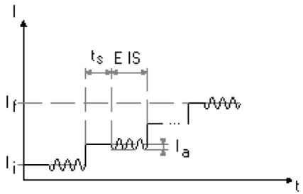
Figure 6: SGEIS technique description.
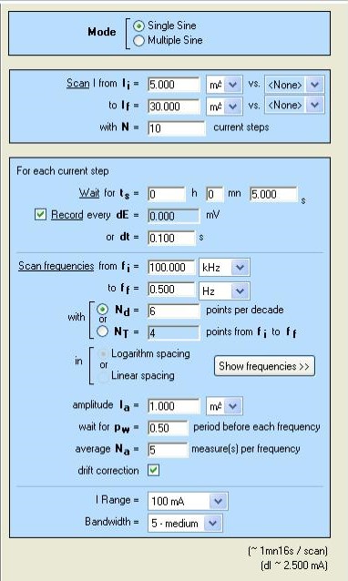
Figure 7: SGEIS technique parameters window.
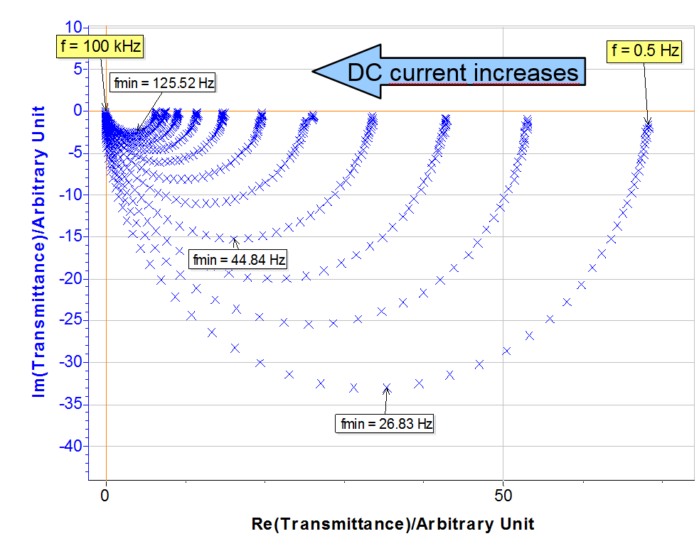
Then, the resulting imaginary part and the real part of the transmittance is plotted in Fig. 8. This plot exhibits for each DC level a capacitive arc which is higher for the low DC level than for the higher one. These arcs are characterized by the minimum frequency of the imaginary part, named fmin.
Higher modulation at 2 mA and 5 mA were performed at the same DC level and exhibit the same behavior.


Figure 8: Nyquist plot of IMVS.
The lifetime of the electron τn is related to the minimum frequency fmin by the following equation [3-5]:
$$\tau n=(2 \pi f_{\text{min}})^{-1} \tag1$$
Assuming that experimental data are obtained with a RC parallel circuit, the minimum frequency can be estimated via the Nyquist plot. But the accurate value of fmin is calculated from the SGEIS data fit carried out with the Zfit tool. The minimum frequency is defined by:
$$f_{min}=(2 \pi \text{RC})^{-1} \tag2$$
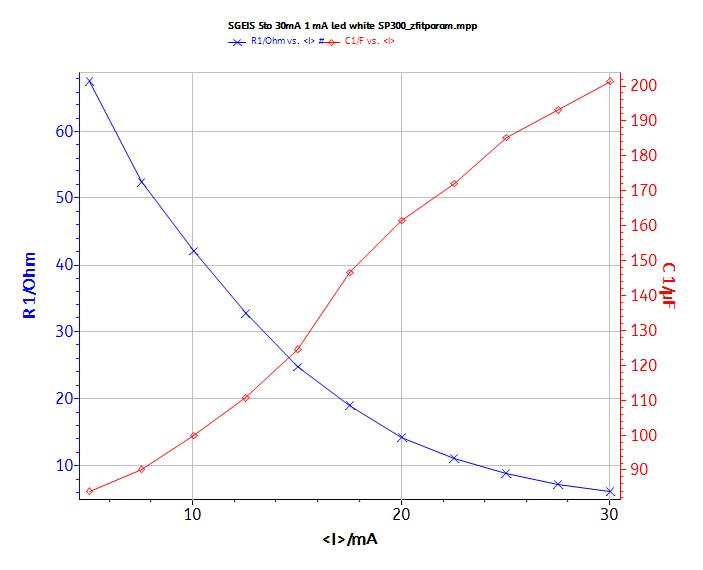
Figure 9: Result of the data fit with a RC parallel circuit.
Because PV cells are more efficient under high illumination, the R1 resistance decreases and the capacitor C1 increases when the light intensity increases (DC level of illumination).
Results of the fit are summarized in Tab. II and Fig. 9.
Table II: Resistance, Capacitor, Minimum frequency and Electron lifetime of white LED vs. light intensity.
| Light intensity/W·m-2 | R/Ohm | C/µF | fmin/Hz | τn/ms |
|---|---|---|---|---|
| 0.500 | 67.55 | 84.04 | 28.05 | 5.94 |
| 0.750 | 52.45 | 90.48 | 33.56 | 4.59 |
| 1.000 | 42.12 | 99.91 | 35.32 | 4.04 |
| 1.250 | 32.84 | 110.78 | 43.77 | 3.55 |
| 1.500 | 24.73 | 124.73 | 51.62 | 3.12 |
| 1.750 | 18.95 | 146.48 | 57.36 | 2.74 |
| 2.000 | 14.27 | 161.35 | 69.20 | 2.41 |
| 2.250 | 11.09 | 172.00 | 83.52 | 1.87 |
| 2.500 | 8.83 | 185.32 | 97.29 | 1.64 |
| 2.749 | 7.22 | 193.07 | 114.30 | 1.45 |
| 2.999 | 6.14 | 201.40 | 128.69 | 1.27 |
From these results, the graph electron lifetime vs. light intensity can be plotted. The relationship between these two variables is characteristic of the kinetic of the electron recombination within the PV cell. The semi-logarithmic plot (Fig. 10) exhibits the “linear” behavior described in the literature [5].
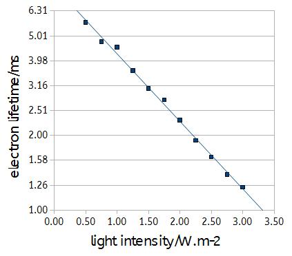
Figure 10: Light intensity vs. electron lifetime.
Conclusion
Transmittance measurements become a standard technique to characterize PV cells, especially IMVS technique.
In this note, we have shown how to perform IMVS techniques with a simple set-up (easy connection, user-friendly software with the appropriate analysis tool).
To complete IMVS investigations, linear polarization and impedance measurements can be achieved. These two techniques are described in a previous application note [6].
Data files can be found in :
C:\Users\xxx\Documents\EC-Lab\Data\Samples\Photovoltaic\AN30_X
References
1) J.-P. Diard, B. Le Gorrec, C. Montella, Cinétique électrochimique, Hermann, Paris (1996) 216.
2) M. E. Orazem, B. Tribollet, Electrochemical Impedance Spectroscopy, Wiley, Hoboken Ch.14 (2008).
3) G. Schlichthorl, S. Y. Huang, J. Sprague, and A. J. Frank, J. Phys. Chem. B, 101 (1997) 8141.
4) T. Oekermann, D. Zhang, T. Yoshida, and H. Minoura, J. Phys. Chem. B, 108 (2004), 2227.
5) J. Bisquert, F. Fabregat-Santiago, I. Mora-Sero, G. Garcia-Belmonte, and S. Gimenez J. Phys. Chem. C, 113 (2009) 17278.
6) Application note #24 “Photovoltaic Characterizations: Polarization and Mott-Schottky plot”
Revised in 08/2019


