

Photovoltaic Characterizations: Polarization and Mott Schottky plot Photovoltaic – Application Note 24
Latest updated: May 5, 2023Abstract
This note describes basic photovoltaic characterization under illumination using the linear polarization (LP) technique. Calculations for short circuit current, open-circuit voltage, fill factor, power and efficiency are presented. In the second part, Mott Schottky measurements are described using the staircase electrochemical impedance spectroscopy (SPEIS) technique. From this, the semiconductor donor density (N) and flat band potential (EFB) are calculated. An equivalent circuit is used to fit the data and extract resistance and capacitance as a function of potential for the photovoltaic.
Introduction
The greenhouse effect and energy price increases has seen the rapid development of new forms of alternative energy.
These include fuel cells, biofuel cells, nuclear, biomass, wind power, and photovoltaic energy sources. Among all these renewable energies, photovoltaic power seems very promising. Indeed, only 0.2% of the solar energy which touched the Earth’s surface will be sufficient to produce energy for the entire planet. [1,2]. A huge amount of research is being carried out in this field in order to improve the efficiency of such an energy supply.
The basic principle of a photovoltaic cell is presented in Figure 1. It is made up of two layers of n-type (electron acceptor) and p-type (electron donor) semiconductors.
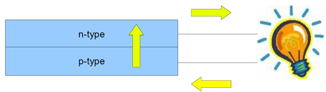
Figure 1: Photovoltaic cell principle.
In this note, several electrochemical investigations are performed in order to characterize the photovoltaic cell, such as I-V characterizations or electrochemical impedance spectroscopy (EIS).
Experimental
Investigations were carried out with the SP-150 driven by EC-Lab® software. The size of the photovoltaic cell was 5.7 x 5.0 cm.
Measurements were performed under natural solar light during a sunny day.
I – E Characterization
Firstly, the photovoltaic cell is characterized by I-V characterization technique (Figure 2).
Note that power is automatically ticked in the “Cell Characteristics” window if I-V characterization technique is selected in the “Photovoltaic/Fuel Cells” part.
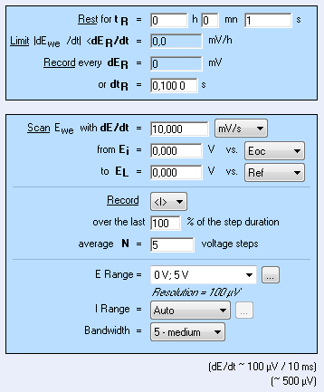
Figure 2: “Parameters settings” window of I-V characterization technique.
The resulting I-V characterization shows a typical I vs. E and P vs. E curves (Figure 3). Several parameters can be drawn from this curve with the “Photovoltaic analysis” tool (Figure 5):
- the Short Circuit Current (Isc), which corresponds to the maximum current when E = 0 V, Isc = 41 mA,
- the Open Circuit Voltage (Eoc), which is the potential when the current is equal to zero ampere, Eoc = 3.145 V,
- the theoretical power (PT), which is defined by the following relationship PT = Isc x Eoc, PT = 129 mW,
- the maximum power, PMAX = 91 mW,
- the fill factor (FF), which is the ratio of PMAX and PT, FF = 70.3%,
- the efficiency can also be calculated. If we assume that the solar power is equal to the means of the solar power per unit of surface (175 W/m2), which is 499 mW for our photovoltaic cell surface area (28.5 cm2). The efficiency of the solar cell is 18%

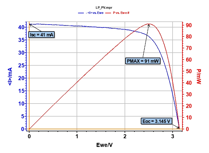
Figure 3: I-V Characterization measurements.
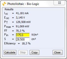
Figure 4: Photovoltaic analysis window.
Impedance Characterization
Mott-Schottky
As photovoltaic cells are made of a semiconductor, the Mott-Schottky plot gives useful information [3-4]. This plot is available from Staircase Potentio Electrochemical Impedance Spectroscopy (SPEIS) investigation. Settings are as follows (Figure 5) and results are given in Fig. 6.
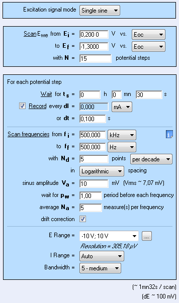
Figure 5: SPEIS settings window.
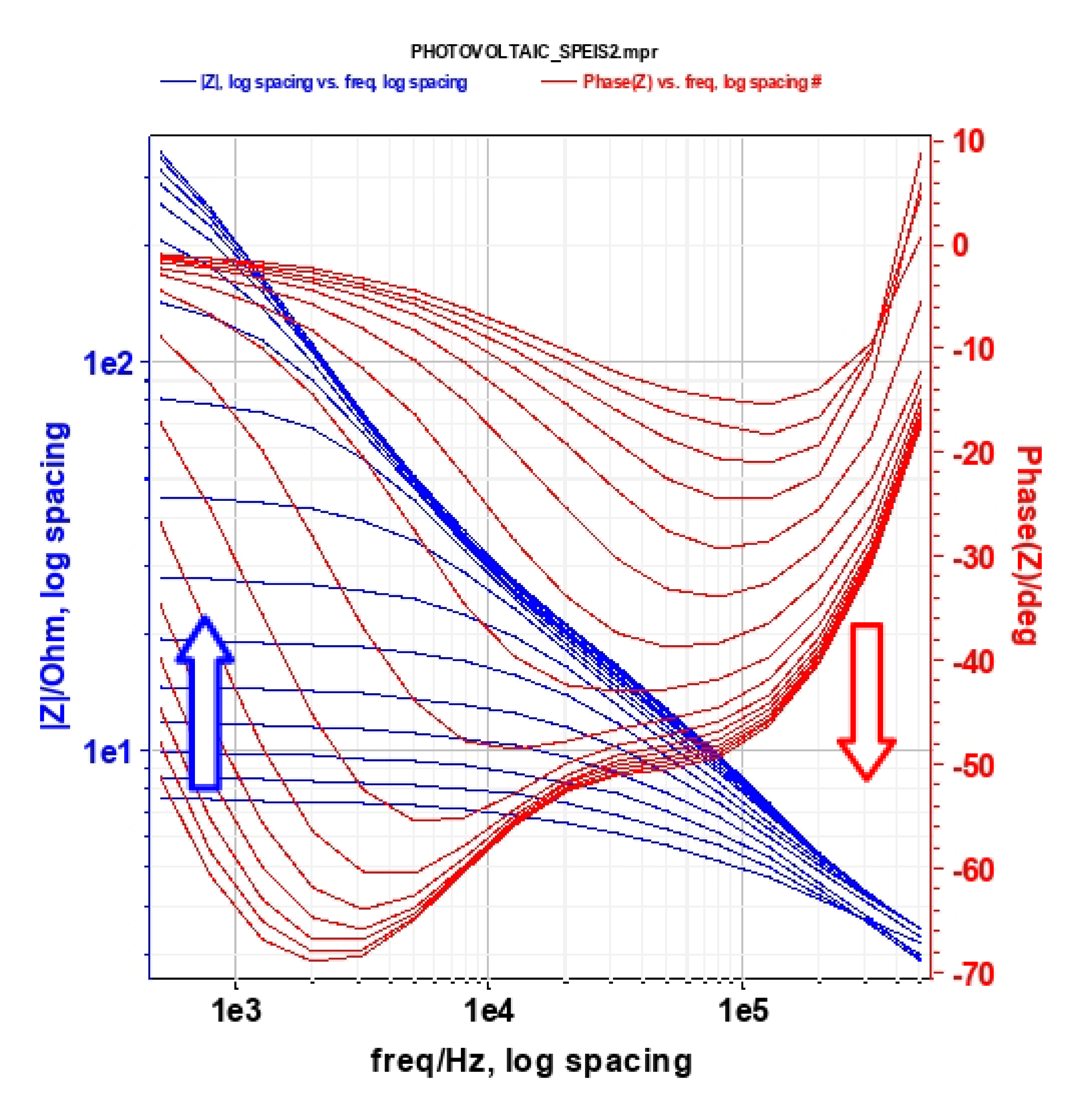
Figure 6: Bode plot of SPEIS investigation. Arrows show the shift of the modulus or phase shift during measurement.
The Mott-Schottky relationship involves the apparent capacitance measurement as a function of potential under depletion condition:
$$\frac{1}{C_{\textrm{sc}}^2}=\frac{2}{e\varepsilon\varepsilon_0N}(E-E_{\textrm{FB}}-\frac{kT}{e}) \tag{1}$$
where Csc is the capacitance of the space charge region, ε is the dielectric constant of the semiconductor, ε0 is the permittivity of free space, N is the donor density (electron donor concentration for an n-type semi-conductor or hole acceptor concentration for a p-type semi-conductor), E is the applied potential, EFB is the flat band potential, k is the Boltzmann Constant, and T is the temperature.
The donor density can be calculated from the slope of the 1/C2 vs. Ewe curve, and the flat band potential can be determined by extrapolation to 1/C = 0. The model required for the calculation is based on two assumptions:
- a) Two capacitances must be considered: the one relating to the space charge region and the one for the double layer. Since capacitances are in series, the total capacitance is the sum of their reciprocals. As the space charge capacitance is much smaller than the double layer capacitance, the double layer capacitance contribution to the total capacitance is negligible. Therefore, the capacitance value calculated from this model is assumed to be the value of the space charge capacitance.
- b) The equivalent circuit used in this model is a series combination of a resistor and a capacitance (the space charge capacitance). The capacitance is calculated from the imaginary component of the impedance (Im(Z)) using the relationship:
$$Im(Z)=\frac{-1}{2\pi fc} \tag{2}$$
This model is adequate if the frequency is high enough (on the order of kHz). For the photovoltaic cell, the frequencies of interest are 200, 50, and 20 kHz (Fig. 6). For a frequency equal to 200 kHz, EFB is 3.204 V, and the donor density is 0.644·1015 cm-3. The negative slope of the Mott-Schottky plot corresponds to a p-type conductivity of the photovoltaic cell.
The straight line in the Mott-Schottky plot is characteristic of the dopant with uniform
distribution within the photovoltaic cell (Fig. 7) [4].
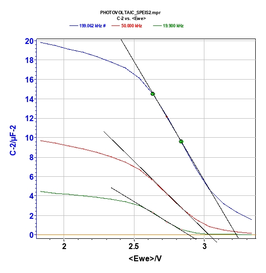
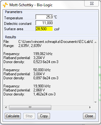
Figure 7: Mott-Schottky plot at frequency of 200 (blue line), 50 (red line), and 20 kHz (green line) (Top) and parameter settings (bottom).
Equivalent Circuit
The equivalent circuit of the photovoltaic cell can be figured by a R1+R2/C2 since one system is observed at around 30 kHz on the Bode plot (phase vs. frequency, in Figure 6) [5]. Fits are performed at several applied potentials thanks to the “Z Fit” [6,7] tool. It is worth noting that fits on all cycles are performed at once automatically by choosing “All” in the select option (Fig. 8).
Nyquist plots (Fig. 7) are typical for this kind of material [8]
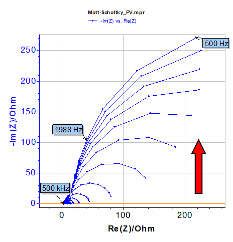
Figure 8: Nyquist plot. The red arrow shows increasing DC potential values.
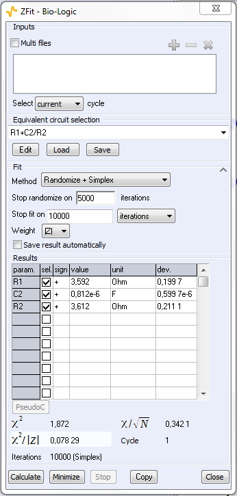
Figure 9: “Z Fit” tool.
The results of an EIS data fit are summarized in Fig. 10. As expected, R1, which corresponds to ohmic resistance, is stable over the potential sweep and R2 decreases when the potential increases. It is important that R2 is also available from the I-E characterization. Indeed, the inverse of the slope of the steady-state curve (I vs. Ewe, Figure 3) is equal to this resistance. Some values are compared in Table I. Both methods give similar results.
Table I: Comparison between R2 determined by I-E and EIS characterization.
| E/V | 2 | 2.5 | 3 |
|---|---|---|---|
| R2/Ω from I – E data | 439 | 74 | 11 |
| R2/Ω from EIS data | 368 | 86 | 9 |
C2 is stable for a potential inferior to 2 V. Then decreases to OCV and finally increases.
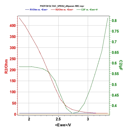
Figure 10: Zfit results with the following equivalent circuit R1+R2/C2.
Conclusion
This note shows the characterization of photovoltaic solar cells by polarization and EIS techniques which allow the user to determine cell performance (Isc, Eoc, PMAX, PT, FF) and model (equivalent circuit).
Moreover, automatic fits on several EIS experiments are available in the “Z Fit” tool. More generally, this note shows the contribution of electrochemistry in energy fields, which is currently a topic of interest.
Data files can be found in:
C:\Users\xxx\Documents\EC-Lab\Data\Samples\Photovoltaic\LP_PV and Mott-Schottky_PV
References
- T. Aartsma, E.-M. Aro, J. Barber, D. Bassani, T. Flüeler, H. de Groot, A. Holzwarth, O. Kruse, A. W. Rutherford,
- European Science Fundation, Science Policy Briefing, n°34 (2008).
- M. Tao, The Electrochemical Society Interface, Winter (2008) 30.
- C.H. Champness, Thin Solid Films, 515(15) (2007) 6200.
- G. Jarosz, J. of Non-crystalline Solids, 354 (2008) 4338.
- N. Ohta, K. Takada, T. Sasaki, M. Watanabe, J. Electrochem. Soc., 152(6) (2005) A1241.
- Application Note #18 “Staircase Potentio Electrochemical Impedance Spectroscopy and automatic successive ZFit analysis”
- Application Note #20 “Pseudo capacitance calculation”
- F. Fabregat-Santiago, J. Bisquert, E. Palomares, L. Otero, D. Kuang, S. Zakeerudin, M. Grätzel, . Phys. Chem., 111 (2007) 6550.
Revised 04/2023


