ZFit and multiple impedance diagram fitting (EIS Zfit) Battery & Corrosion – Application Note 45

Introduction

Electrochemical impedance spectroscopy (EIS) measurements are widely implemented in all fields of electrochemistry (e.g. energy and corrosion applications). The impedance diagrams are usually fitted using equivalent electrical circuits (EC) [1-3]. Variations of EIS measurements are frequently linked with physical parameters, like potential or temperature. This behavior results in variations of the values of EC parameters. The analysis of EIS measurements at different conditions becomes important to understand the system of interest’s physical behavior [1, 2].
In this context, EC-Lab^® provides a powerful and user-friendly tool to fit successive EIS diagrams called ZFit. ZFit automatically determines (and plots) successive values of EC components for a series of impedance diagrams. This advanced feature allows the user to model experimental results [4].
SPEIS and SGEIS techniques allow the user to perform successive impedance measurements. Application Note # 17 describes the use of SPEIS technique and ZFit [5] tools in order to fit the presented EIS diagram.
This note explains the use of ZFit to adjust the component values of EC, for several impedance diagrams. The different options to fit several EIS diagrams are also presented. Examples in batteries, photovoltaic cells and corrosion application are shown to illustrate the functionalities of ZFit.

Fitting Multiple Impedance Diagrams

ZFit allows users to choose an equivalent circuit in a list of predefined circuits or edit a new EC if it is not in this list¹. Equivalent Circuit edition windows of ZFit is shown in Fig. 1.

Figure 1: Equivalent Circuit Edition window.

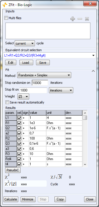
In order to fit multiple EIS graphs, the user must first, select (or create) the EC in the Equivalent Circuit block, and choose Select “all” cycles in the ZFit windows (Fig. 2) in the Fit block.
ZFit provides three minimization algorithms: Randomize, Simplex and Levenberg-Marquardt. The user can combine Randomize with Simplex or Levenberg-Marquardt. Using the Randomize option is better to provide automatically suitable initial values for further minimizations. If Randomize + Simplex or Randomize + Levenberg-Marquardt option are selected, the Randomize minimization could be performed on the first cycle only or on every cycle. If the parameters are close (between the successive cycles), it is recommended to use the Randomize option only in the first cycle. The user can choose the maximum number of Randomization iterations.

Figure 2: ZFit window.

The evolution of fitted EC parameters are automatically displayed in a new graph.

Experimental Results

Li-Ion Batteries Application: SOC and SOH

The EIS technique was used to study the state of charge or state of health (SOC or SOH) of batteries. EIS is a non-destructive, fast and easy-to-use technique. The variation of EIS diagrams (EC parameters) would enable the determination of SOC and SOH [2]. In the present note, the EIS measurements on a commercial Li-ion battery are presented (nominal capacity 2.4 Ah). The EIS diagrams were analyzed using ZFit.
The Nyquist diagrams were obtained using PEIS protocol (Fig. 3). Each diagram was measured after a discharge at C/10 rate for 30 min, followed by 10 min at open circuit potential, OCV (GCPL technique). One can observe the two typical capacitive circle arcs at high and middle frequencies (attributed respectively to the solid electrolyte interphase (SEI) and the charge transfer). At low frequencies one can highlight a diffusion region.

Figure 3: Results of fitting process with ZFit.

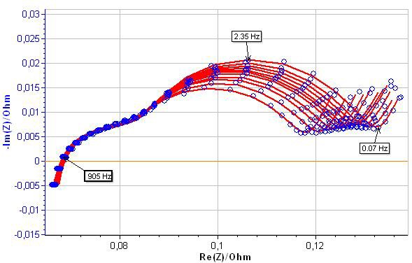
The EIS graphs have been fitted with the EC: L1+R1+Q2/(R2+Q3/R3)+Q4 (Fig. 4). The results of the fitting process are also shown in Fig. 3.

Figure 4:  Equivalent circuit used to fit the experimental result from Fig. 3

As mentioned above, one can use ZFit to study the evolution of EC parameters. Fig. 5 shows the evolution of internal resistance R1, SEI and charge transfer associated resistances (R2 and R3, respectively) with the potential.

Figure 5: Evolution of R1 (□), R2 (○) and R3 (∆) with the potential.

In the battery field, these values are valuable and can be used to characterize and further determine batteries’ state of charge (SOC) or state of health (SOH) [1-3, 5].

Photovoltaic Cells Application

Silicon solar cells can be characterized by plotting polarization curves and measuring impedance at several points of the curve [6, 7].
The photovoltaic cell (PV) was characterized under white-LED constant illumination. The EIS measurements have been performed under potential control (SPEIS technique) between 0 and 3.8 V every 200 mV. The results of these measurements are shown in Fig 6.

Figure 6: Results of SPEIS measurements on a PV cell.

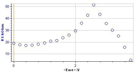
These EIS graphs can be, in a first approximation, fitted by a R/C circuit. The evolution of the resistance with the potential is shown in Fig.8. R1 value reaches a maximum value at 2.6 V.

Figure 7: Results of fitting process with ZFit.

Figure 8: Evolution of resistance R1 with the potential.

Corrosion: Polarization Resistance Evolution As A Function Of Time

The corrosion current can be determined by measuring the polarization resistance, (R_p), at the corrosion potential by using the Stern-Geary relationship [9, 10]. Stationary (voltammetry at low scan rate) or dynamic measurements (EIS) can be performed to determine the R_p value.
The corrosion rate variations, as a function of time, are particularly useful in the chemical industry to evaluate for instance the influence of experimental conditions in a reactor (addition of a reagent, temperature, etc.).
In this note, we present the EIS measurements performed (under potential control) on an AISI 108 steel sample in 0.5 M H₂SO_4. The electrode surface was slightly passivated applying 1V v.s. SCE during 1 s. EIS measurements  were  carried  out  at  the corrosion potential. The EIS diagrams obtained are shown in Fig 9. The EC: La1+R1+C2/R2 was used to fit the experimental results (where R2 corresponds to R_p) (Fig.10).

Figure 9: EIS measurements on AISI 108 steel sample (blue points) and results of fitting process with ZFit (dashed red line).

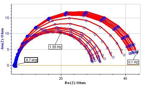
Figure 11 shows the evolution of R_p during the passivation process. One can observe the non-monotonic variation of R_p with the cycle number (equivalent to time). Between the first and third cycle, the R_p value decreases. Then, the value increases up to the twelfth cycle. After that, the R_p value slightly decreases.

Figure 10: Equivalent circuit use to fit the experimental result from Fig. 9.

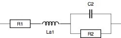
Figure 11: Evolution of the polarization resistance with the number of cycles (time).

References

[1] F. Huet. J. Power Sources, 70 (1998) 59.
[2] U. Tröltzsch, O. Kanoun, and H.-R. Tränkler. Electrochim. Acta, 51 (2006) 1664.
[3] J.-P. Diard, B. Le Gorrec, and C. Montella. J. Power Sources, 78 (1998) 78.
[4] A. Pellissier, N. Portail, N. Murer, B. Molina- Concha, S. Benoit, and J.-P. Diard. ZFit: a powerful tool for multiple impedance diagram fitting. EIS2013-9th International Symposium on Electrochemical Impedance Spectroscopy, poster (Okinawa, Japan), 2013.
[5] Application note #17 “Staircase Potentio Electrochemical Impedance Spectroscopy and automatic successive ZFit analysis.”
[6] M. Keddam, Z. Stoynov, and H. Takenouti. J. App. Electrochem., 7 (1977) 539.
[7] D. Chenvidhya, K. Kirtikara, and C. Jivacate. Sol. Energy Mater. Sol. Cells, 80 (2003) 459.
[8] F. Fabregat-Santiago, J. Bisquert, G. Garcia- Belmonte, G. Boschloo, and A. Hagfeldt. Sol. Energy Mater. Sol. Cells, 87 (2005) 117.
[9] M. Stern and A. L. Geary. J. Electrochem. Soc., 104 (1957) 56.
[10] M. Prazak and K. Barton. Corrosion Science, 7 (1967) 159.
Revised in 08/2019
1 ZFit has 13 components to build the equivalents circuits. Among them, there are the specific electrochemical elements, such as Wδ (diffusion-convection) or M (restricted linear diffusion).