How to fit transmission lines with ZFit (EIS transmission lines) Battery – Application Note 43
Latest updated: April 2, 2025Abstract
This application note describes how to fit transmission lines using one equivalent circuit elements contained in Z Fit. For example, the Warburg impedance is equivalent to that of a semi-infinite large network i.e. a transmission line.
Introduction
ZFit is the EC-Lab® impedance fitting tool. This note will describe how to fit transmission lines using one equivalent circuit elements contained in ZFit.
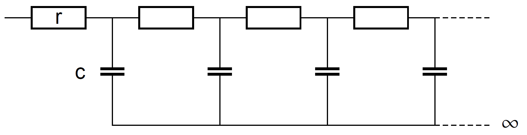
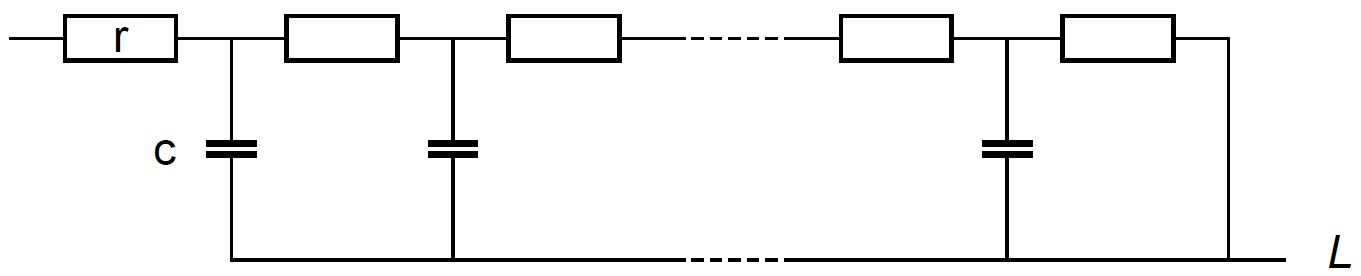
It has long been known that the Warburg impedance is equivalent to that of a semi-infinite large network i.e. a transmission line, as shown in Fig. 1 [1, 2].

Figure 1: The equivalent circuit of the Warburg impedance.
More recently it has been shown [3] that the impedance of a L-long transmission line made of χ and ζ elements and terminated by a ZL element (Fig. 2) is given by the general expression:

Figure 2: Uniform transmission line made χ and ζ elements and terminated by ZL [3].
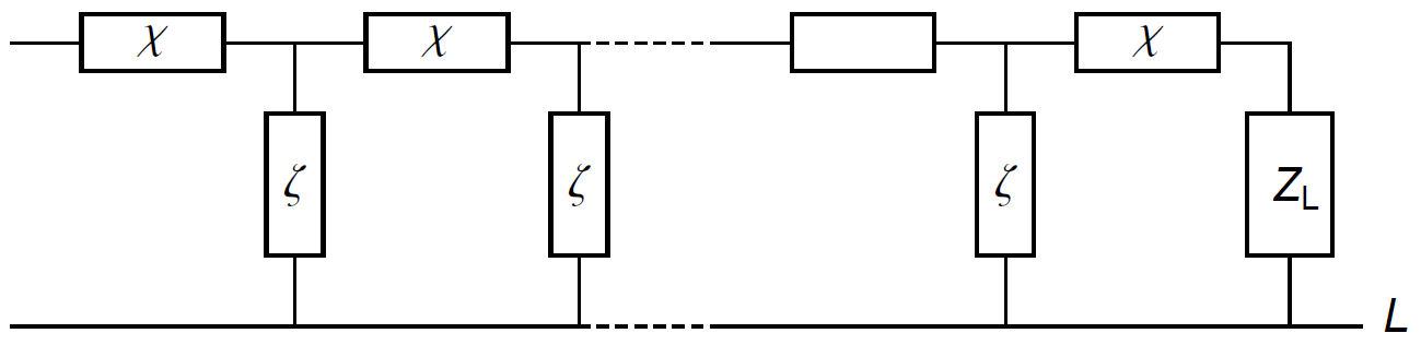
$$Z= \frac{(\zeta \chi – Z_\text L^2) \text{sh} \left(\frac{L\sqrt{\chi}}{\sqrt{\zeta}} \right)}{{Z_\text L \; \text{sh} \left(\frac{L\sqrt{\chi}}{\sqrt{\zeta}} \right)}+ \sqrt{\zeta \chi} \; \text{ch} \left(\frac{L\sqrt{\chi}}{\sqrt{\zeta}} \right)} + Z_\text L$$
With three limiting cases
– open-circuited transmission line
$$Z_\text L = \infty \Rightarrow Z= \sqrt{\zeta \chi}\; \text{coth} \left(\frac{L \sqrt{\chi}}{\sqrt{\zeta}} \right) \tag{1}$$
– short-circuited transmission line
$$Z_\text L = 0 \Rightarrow Z= \sqrt{\zeta \chi} \text{th} \left(\frac{L \sqrt{\chi}}{\sqrt{\zeta}} \right) \tag{2}$$
– semi-infinite transmission line
$$L \rightarrow \infty \Rightarrow Z = \sqrt{\zeta \chi} \tag{3}$$
Hereafter, some transmission lines are described and the corresponding ”simple” equivalent circuit elements are shown. Firstly, the open-circuited transmission lines will be explained, followed by short-circuited and semi-infinite transmission lines.
OPEN-CIRCUITED TRANSMISSION LINES $Z_\text L =1$
OPEN-CIRCUITED URC (UNIFORM DISTRIBUTED RC)
Let us consider the open-circuited transmission line made of r and c elements (Fig. 3).

Figure 3: L-long open uniform distributed RC (URC) transmission line [4,5].
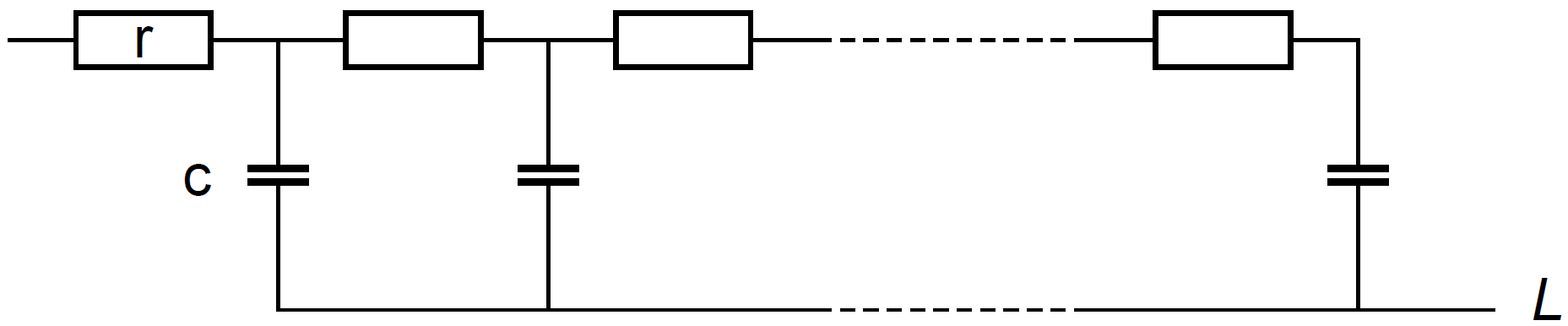
Using Eq. (1), the transmission line impedance is given by:
$$\chi = r, \zeta = \frac{1}{j \omega c} \Rightarrow Z = \sqrt{r} \frac{\text {coth}(L\sqrt{rcj \omega})}{\sqrt{cj \omega}} \tag{4}$$
With ω = 2πf. This impedance is similar to that of the M element of ZFit
$$Z_\text M = R_\text d \frac{\text{coth}\sqrt{\tau_\text d j \omega}}{\sqrt{\tau_\text d j \omega}}, R_\text d = L_\text r, \tau_ \text d = L^2rc \tag{5}$$
OPEN-CIRCUITED URQ
Replacing c elements by q elements, with $Z_\text q = 1/(q(j \omega)^\alpha)$ leads to transmission line shown in Fig. 4.

Figure 4: L-long open uniform distributed RQ|(URQ) transmission line.

The transmission line impedance is given by
$$\chi = r, \zeta = \frac{1}{q(j \omega)^\alpha} \Rightarrow Z = \sqrt{r} \frac{\text{coth} \left(L\sqrt{rq}(j \omega)^{\alpha/2} \right)}{\sqrt{q}(j \omega)^{\alpha/2}} \tag{6}$$
The impedance is similar to that of the Ma element of ZFit.
$$Z_{\text{M_a}} =R \frac{\text{coth}(\tau j \omega)^{\alpha/2}}{(\tau j \omega)^{\alpha/2}} \tag{7}$$
With
$R = Lr, \tau = (L^2rq)^{1/\alpha}$
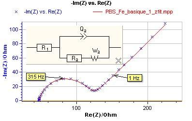
For example, a Nyquist impedance diagram of a battery Ni-MH 1900 mAh is shown in Fig. 5. The equivalent circuit R1+L1+Q1/(R2+Ma3), containing a Ma element, is chosen to fit the data shown in Fig. 5. The values of the parameters, obtained using the EC-Lab ZFit tool , are R1 = 0.049 Ω, L1 = 0.154 10−6 H, Q1 = 0.66 F sα−1, α1 = 0.61, R2 = 0.0236 Ω, R3 = L r = 0.057 Ω, τ3 = (L2 r q)1/α = 2.25 s and α3 = 0.89.

Figure 5: Nyquist impedance diagram of a battery Ni-MH 1900 mAh.
The equivalent circuit of the anomalous diffusion is shown in Fig. 6 [6].

Figure 6: L-long open uniform distributed QC (UQC) transmission line. Anomalous diffusion [6].

The anomalous diffusion impedance is given by
$$\chi = \frac{1}{q (j \omega)^\alpha}, \zeta = \frac{1}{cj \omega} \Rightarrow Z = \frac{\text{coth} \left(L\sqrt{\frac{c}{q}}(j \omega)^{\frac{1}{2} – \frac{\alpha}{2}} \right)}{\sqrt{cq}(j \omega)^{\frac{\alpha}{2}+\frac{1}{2}}} \tag{8}$$
This impedance is similar to that of the Mg element of ZFit
$$Z_{\text{M_g}} =R \frac{\text{coth}(\tau j \omega)^{\gamma/2}}{(\tau j \omega)^{1-\gamma/2}} \tag{9}$$
With $\gamma = 1- \alpha$, $R= c^{\frac{1}{\gamma}-1}\; L^{\frac{2}{\gamma}}\; q^{\frac{-1}{\gamma}},\; \tau = c^{\frac{1}{\gamma}-1}\; L^{\frac{2}{\gamma}}\; q^{\frac{-1}{\gamma}}$
SHORT-CIRCUITED TRANSMISSION LINES $Z_\text L = 0$
SHORT-CIRCUITED URC

Figure 7: L-long open uniform distributed RC (URC) transmission line.
Using Eq. (2), the impedance of the short-circuited transmission line made of r and c elements (Fig. 7) is given by
$$\chi = r, \zeta = \frac{1}{cj \omega} \Rightarrow Z = r \frac{\text{th}(L\sqrt{rcj \omega)}}{\sqrt{rcj \omega}} \tag{10}$$
This impedance is similar to that of the Wd element of ZFit
$$Z_\text{W_d} = R_\text{d} \frac{\text{th}\sqrt{\tau_\text{d}j \omega}}{\sqrt{\tau_\text{d}j \omega}},R_\text{d} = Lr,\tau_\text{d} = L^2rc \tag{11}$$
SEMI-INFINITE TRANSMISSION LINES: $L \rightarrow \infty$
SEMI-INFINITE URC
The impedance of the semi-infinite transmission line shown in Fig. 1 is obtained making in Eq. (10).
$$L \rightarrow \infty \Rightarrow Z = r \frac{\text{th}(L\sqrt{rcj \omega})}{\sqrt{\sqrt{rcj \omega}}} \approx \frac{\sqrt{r}}{\sqrt{cj \omega}} \tag{12}$$
This expression is similar to that of the Warburg (W) element of ZFit
$$Z_\text{W} = \frac{2\sigma}{\sqrt{j\omega}} \, \text{with} \, \sigma = \frac{\sqrt{r}}{2\sqrt{c}} \tag{13}$$
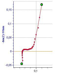
As an example a Nyquist impedance diagram of a Fe(II)/Fe(III) system is shown in Fig. 8.

Figure 8: Nyquist impedance diagram of a Fe(III)/Fe(II) system in basic medium.
The Randles circuit R1+Q2/(R2+W2), containing a Warburg element, is chosen to fit the data shown in Fig. 8. The values of the parameters for equivalent circuit are R1 = 47.57 Ω, Q2 = 17.09 x 10⁻⁶ F s-1, α = 0.885, R2 = 70.94 Ω and σ2 = 85.33 Ω s-1/2 Ω s-1/2.
$\Rightarrow \sqrt{\frac{r}{c}}$ = 42.7 Ω s-1/2
SEMI-INFINITE URRC
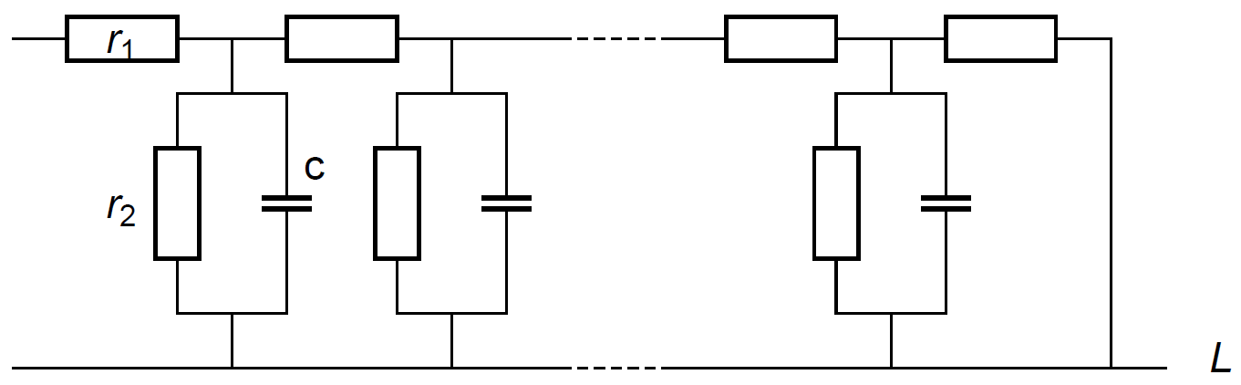
First of all, let us calculate the impedance of the L-long URRC transmission line (Fig. 9) corresponding to diffusion-reaction and diffusion-trapping impedance [7]:

Figure 9: L-long short-circuited uniform distributed RRC (URRC) transmission line.
$$\chi = r_1, \zeta = \frac{r_2}{1+r_2cj \omega} \Rightarrow Z = \sqrt{r_1r_2} \frac{\text{th}\left(L\sqrt{\frac{r1}{r2}(1+r_2cj \omega})\right)}{\sqrt{1+r_2cj \omega}} \tag{14}$$
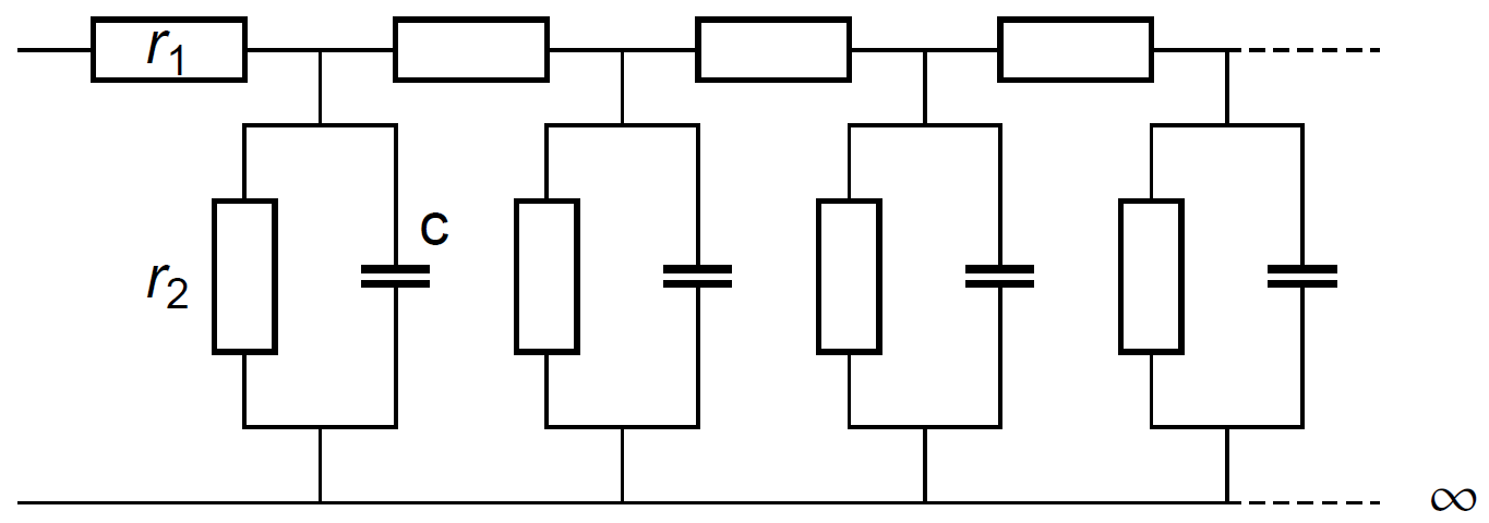
Figure 10: Semi-infinite short-circuited uniform distributed RRC (URRC) transmission line.
With it is obtained [8]:
$$L \rightarrow \infty \Rightarrow Z \approx \frac{\sqrt{r_1r_2}}{\sqrt{1+r_2cj \omega}} \tag{15}$$
This expression is similar to that of the Gerischer element G of ZFit [9]:
$$Z_\text{G}= \frac{R_\text G}{\sqrt{1 + \tau_\text G J \omega}},R_\text G = \sqrt{r_1r_2}, \tau_\text G = r_2c \tag{16}$$
SEMI-INFINITE URRQ

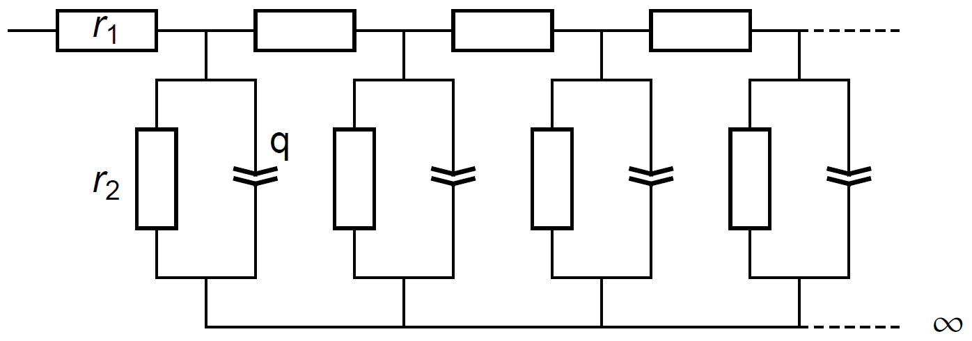
Figure 11: L-long short-circuited uniform distributed RRQ (URRQ) transmission line.

Replacing c elements by q elements
$$\chi = r_1, \zeta = \frac{r_2}{1+r_2c(j \omega)^{\alpha}} \Rightarrow Z = \sqrt{r_1r_2} \frac{\text{th}\left(L\sqrt{\frac{r1}{r2}(1+r_2c(j \omega})^{\alpha})\right)}{\sqrt{1+r_2c(j \omega)^{\alpha}}} \tag{17}$$

Figure 12: Semi-infinite short-circuited uniform distributed RRQ (URRQ) transmission line.
And
$$L \rightarrow \infty \Rightarrow Z \approx \frac{\sqrt{r_1r_2}}{\sqrt{1+\tau(j \omega)^{\alpha}}} \tag{18}$$
This expression is similar to that of the Ga element of ZFit
$$Z_\text{G_a}= \frac{R}{\sqrt{1 + \tau(j \omega)^{\alpha}}} , R = \sqrt{r_1r_2} , \tau=r_2q \tag{19}$$
Conclusion
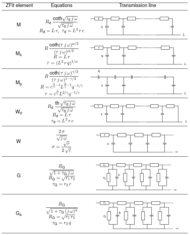
Seven elements, W, Wd, M, Ma, Mg, G and Ga, available in ZFit correspond to different transmission lines (Tabs. I and II).
Table I: Summary table.
| Transmission line | ZFit Element | |
|---|---|---|
| Open Circuited | URC URQ UQC | M Ma Mg |
| Short circuited | URC | Wd |
| Semi-infinite | URC URRC URRQ | W G Ga |
Data files can be found in :
C:\Users\xxx\Documents\EC-Lab\Data\Samples\EIS\PEIS_Fe_Basique_1 and AN43_peis_batteries_carouf_01_PEIS_C06
References
1) J. C. Wang, J. Electrochem. Soc., 134 (1987) 1915.
2) M. Sluyters-Rehbach, Pure & Appl. Chem., 66 (1994) 1831.
3) J. Bisquert, Phys. Chem. Chem. Phys., 2 (2000) 4185.
4) G. C. Temes and J. W. Lapatra, Introduction to Circuits Synthesis and Design, McGraw-Hill, New-York, 1977.
5) J.-P. Diard, B. Le Gorrec, and C. Montella, J. Electroanal. Chem., 471 (1999) 126.
6) J. Bisquert and A. Compte, J. Electroanal. Chem., 499 (2001) 112.
7) J.-P. Diard and C. Montella, J. Electroanal. Chem., 557 (2003) 19.
8) B. A. Boukamp and H. J.-M. Bouwmeester, Solid State Ionics 157 (2003) 29.
9) H. Gerischer, Z. Physik. Chem. (Leipzig), 198 (1951) 286.
Revised in 11/2018
Table II: ZFit elements vs. transmission lines