Two questions about Kramers-Kronig transformations (EIS Kramers-Kronig) Battery – Application Note 15

Using the Kramers-Kronig (KK) transforms, the real part of a transfer function can be calculated for a causal, stable, linear time invariant and finite system when $f \rightarrow\ 0$ and $f \rightarrow\ \infty$, when the change in its imaginary part, as a function of the frequency, is known. Alternatively, the imaginary part of a transfer function can be calculated when the evolution of its real part is known [1-4]. When the impedance of an electrode reaction is measured, it is possible to calculate the imaginary part using experimental values for the real part and calculate the real part using experimental values for the imaginary part. Comparing calculated impedance with the experimental impedance  is a useful tool to check the validity of the impedance measurement with respect to the conditions of applicability of KK transforms.

Figure 1: Test Box-3, test circuit #3. I vs. E_WE steady-state curve.

As an example, the Nyquist impedance diagram shown in Figure 2 has been measured for circuit #3 of the BioLogic Test Box-3 using the PEIS technique. Test circuit #3 mainly consists of two transistors. It is a model for metal passivation [5,6]. The Nyquist impedance diagram shown in Figure 2 is made of two capacitive arcs well separated in frequency. The calculated impedance Z_KK using KK transforms is shown in the Fig. 2.

Z and Z_KK diagrams are similar for all frequencies, therefore impedance measurements have been carried out for a causal, stable, linear and time invariant system.

Figure 2: Test circuit #3. Nyquist impedance diagram measured at point a (Figure 1) using PEIS technique. E_WE = -0.35 V, V_a = 10 mV, f_min = 0.2 Hz, f_max = 50 kHz (blue markers) and Nyquist diagram obtained using KK transforms (red curve).

The Nyquist impedance diagram shown in Figure 3 has been measured using a large value of potential amplitude (V_a = 375 mV) of the sinusoidal modulation of potential E_WE, i.e. for non-linear conditions. This diagram is still made of two capacitive arcs, the low frequency arc being smaller than the corresponding arc in the case of Figure 2.

The calculated impedance Z_KK using KK transforms is shown in Figure 3. These two impedance diagrams are different, showing that the impedance measurement has been carried out for non-linear conditions.

Figure 3: Test circuit #3. Nyquist impedance diagram measured using PEIS technique. E_WE = -0.35 V, V_a = 375 mV, f_min = 0.2 Hz, f_max = 50 kHz (blue markers) and Nyquist impedance diagram obtained using KK transforms (red curve).

Let us suppose that, for some reason, the Nyquist diagram has been measured for a limited-range frequency values (Figure 4).

Figure 4: Truncated impedance diagram obtained for limited-range frequency values. E_WE= 0.35 V, V_a = 10 mV, f_min = 10 Hz, f_max = 50 kHz (blue curve) and Nyquist diagram obtained using KK transforms (red curve).

Obviously Z and Z_KK impedance diagrams show a large discrepancy. What can we do to check the validity of the experimental impedance diagram shown in Figure 4? It is always possible to check this validity using ZFit [6] with a measurement model, i.e. a Voigt circuit R1+C2/R2+C3/R3. As the measurement model is consistent with the KK relations, it allows the user to check the consistency of experimental data without using the KK relationships [7]. The theoretical impedance shown in Figure 5 shows the validity of the truncated experimental impedance diagram.

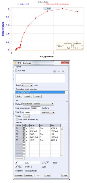
Figure 5: Truncated impedance diagram obtained for limited-range frequency values (blue curve), ZFit window for Voigt circuit R1+C2/R2+C3/R3 and theoretical impedance diagram (red curve).

Test Box-3 Circuit 3

The Nyquist impedance diagram shown in Figure 6 has been measured at point b of the steady-state curve (Figure 1) of circuit #3 of the BioLogic Test Box-3 using the PEIS technique, i.e. under potential control (PC). The Nyquist impedance diagram shown in Figure 6 is still made of two capacitive arcs, well separated in frequency with a negative value of the real part of the impedance in low frequency, according to the bell-shaped steady-state curve.

Figure 6: Test circuit #3. Nyquist impedance diagram measured at point b (Figure 1) using PEIS technique. E_WE = 1.35 V, Va = 10 mV, f_min = 1 Hz, f_max = 100 kHz (blue markers) and Nyquist impedance diagram obtained using KK transforms (red curve).

The result of the KK transform (Figure 6) shows a large discrepancy in the low frequency domain. It has been shown [8,9] that it is not possible to directly verify the validity of an impedance diagram measurement of an “unstable” electrochemical system, such as it would be found, for instance, in the case of a steady-state current density vs. electrode potential curve exhibiting a part with a negative slope. In fact, the KK transforms do not really fail. The bell-shaped curve steady-state current vs. potential curve shown in Figure 1 cannot be entirely drawn under galvanostatic control (GC), whereas it could under potentiostatic control (PC). Gabrielli et al. [9] have demonstrated that, in this case, it was possible to calculate the admittance and then verify the validity of the admittance using KK transforms.

Figure 7: Sketch of the study of a scalar linear system under potentiostatic control (PC).

This problem is due to the electrochemist’s bad habit of working under potentiostatic control (PC) and plotting the impedance diagram instead of an admittance diagram. Under PC, the transfer function H(s) of a system is not impedance but admittance. In fact, a transfer function is given by Figure 7:

$$H(s) = \frac{\mathrm{L[output}(t)]}{\mathrm{L[input}(t)]} \tag{1}$$

Where s is the Laplace variable and L denotes the Laplace transform. Under PC, the transfer function of an electrochemical system is:

$$H(s) = \frac{\mathrm{L}[\Delta I(t)]}{\mathrm{L}[\Delta E(t)]} = \frac{1}{Z(s)} = Y(s) \tag{2}$$

Therefore, checking the consistency of the experimental impedance diagram shown in Figure 6 should be made with admittance data instead of impedance data. Figure 8 shows good agreement between Y and Y_KK admittance diagrams and the consistency of the measured impedance.

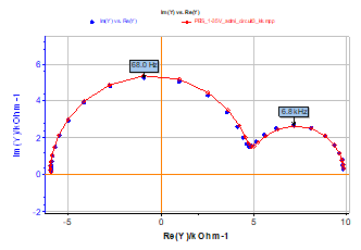
Figure 8: Test circuit #3. Nyquist admittance diagram measured using PEIS technique. E_WE = 1.35 V, V_a= 10 mV,  f_min = 1 Hz,  f_max = 100 kHz (blue markers) and Nyquist admittance diagram obtained using KK transforms (red curve).

To conclude, it is therefore possible to transform Y_KK admittance diagrams into Z_KK impedance diagrams as it is shown in Fig. 9.

Figure 9: Z (blue markers) and Z_KK (red curve) impedance diagrams obtained by inverting admittance diagrams shown in Figure 8.

Ni Electrode in Acidic Medium

The well-known impedance diagram obtained for Ni electrode in H₂SO₄ medium using the PEIS technique is shown in Fig. 10 [10,11]. Such diagrams are obtained for anodic dissolution-passivation of Ni under PC in the instability range of the electrode|electrolyte interface with respect to current control. The impedance diagram is made of two parts, a near semi-circle in the high frequency domain and a near circle arc in the low frequency domain. Obviously, the Z and Z_KK Nyquist diagrams are quite different, and the experimental impedance Z does not obey the KK relationships.

Figure 10: Ni electrode in acidic medium (H₂SO₄ 1 mol·L^‑1, Φ = 2 mm). Nyquist impedance diagram measured using PEIS technique. E_WE = 0.9 V/ECS, V_a = 12.5 mV,  f_min = 50 mHz, f_max = 10 kHz with 25 points per decade (blue markers) and Nyquist diagram obtained using KK transforms (red curve).

Figure 11 shows the good agreement between Y and Y_KK admittance diagrams and the consistency of the measured impedance of Ni electrode in acidic medium. The shift between the admittance diagrams is due to the measurement error of the real part of the impedance for $f \rightarrow\ \infty$.

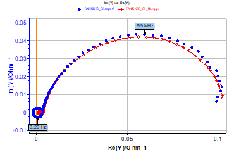
Figure 11: Ni electrode in acidic medium (H₂SO₄ 1 mol·L^‑1, Φ = 2 mm). Nyquist admittance diagram measured using PEIS technique. E_WE = 0.9 V/ECS, V_a= 12.5 mV, f_min= 50 mHz, f_max = 10 kHz with 25 points per decade (blue markers) and Nyquist admittance diagram obtained using KK transforms (red curve).

References

- V. A. Tyagay, G. Y. Kolbasov, Elektrokhimiya, 8 (1972) 59.
- R. L. V. Meirhaeghe, E. C. Dutoit, F. Cardon, W. P Gomes, Electrochim. Acta, 21 (1976), 39.
- J.-P. Diard, P. Landaud, J.-M. Le Canut, B. Le Gorrec, C. Montella, Electrochim. Acta, 39 (1994) 2585.
- A. Sadkowski, M. Dolata, J.-P. Diard, J. Electrochem. Soc., 151 (1) E20-E31.
- Application Note #9 “Linear vs non linear systems in impedance measurements”
- Application Note #14 “Zfit and equivalent electrical circuits”
- P. K. Shukla, M. E. Orazem, O . D. Crisalle, Electrochim. Acta, 49 (2004) 2881.
- D. D. MacDonald, Electrochim. Acta, 35 (1990) 1509.
- C. Gabrielli, M. Keddam, H. Takenouti, Proc. 5th Electrochemical Impedance Forum, Montrouge (1991).
- I. Epelboin, M. Keddam, M.-C. Petit, Electrochim. Acta, 17 (1972) 177.
- F. Berthier, J.-P. Diard, B. Le Gorrec, C. Montella, J. Electroanal. Chem., 572 (2004) 267.
Revised in 07/2018