Equivalent model of electrochemical cell inc. ref. electrode impedance and potentiostat parasitics Battery – Application Note 44

EIS Basics

Introduction

As a non-intrusive and highly sensitive technique, electrochemical impedance spectroscopy (EIS) requires basic, often overlooked or ignored precautions, in order to obtain reliable results. High impedance cells are more sensitive to capacitive artifacts while low impedance cells are more sensitive to inductive and resistive artifacts. Artifacts are even more important as the frequency of analysis now tends to cross the megahertz boundary. Ignoring these artifacts can lead to misinterpretation of results. In this note we focus on the influence of stray capacitances introduced by instrumentation. We also show that the strange results obtained with a poor reference electrode data can be perfectly explained by a complete cell model that includes instrument artifacts.

An Analysis Dilemma

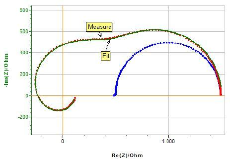
Impedance measurement results are analyzed and compared to simulated data generated from mathematical or electrical models. Model parameters are obtained from a data fitting process. Important differences between measured and simulated data can have two causes: either a wrong or incomplete model or an experimental artifact (Fig. 1).

Figure 1 : Analysis dilemma, measured and simulated data do not match.

How do you identify the origin of these differences? Is it a modeling or a measurement problem? Solving this analysis dilemma requires an awareness of possible measurement artifacts.

Table I: True, effective and measured values.

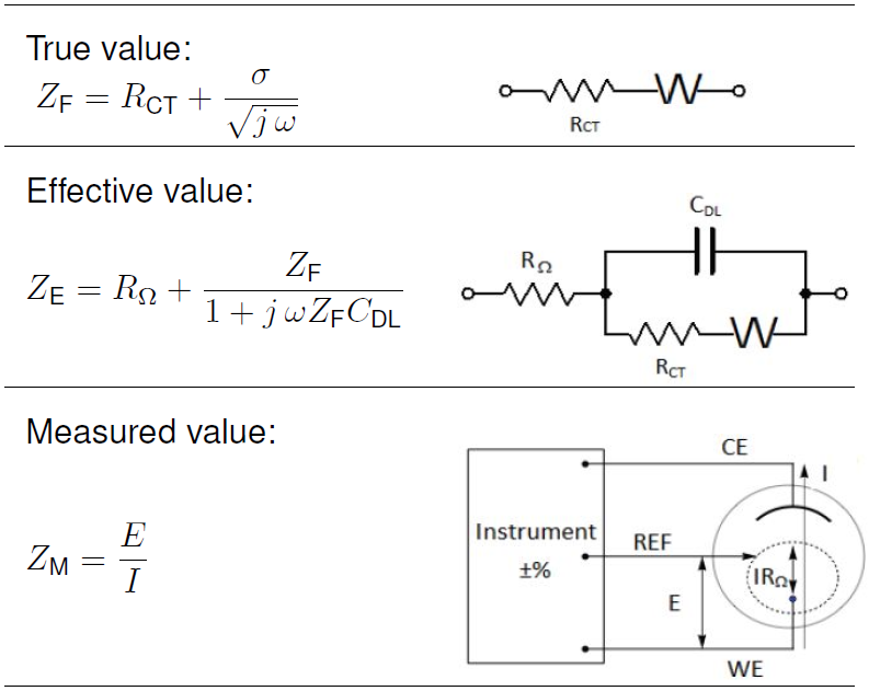
Important differences exist between the true, effective and measured value of an electrochemical impedance. In Tab. I, the true value is the impedance of a basic redox reaction with a semi-infinite diffusion condition. The equivalent electrical model consists of a charge transfer resistance (R_CT) in series with a Warburg diffusional element (W). Generally, the true value is the value of interest but it does not take into account parasitics.
The effective value adds to the true value the elements that cannot be avoided in a measurement. In our example, these elements are the double layer capacitance (C_DL)and the uncompensated solution resistance (R_Ω) related to the electrochemical cell.
The measured or indicated value is the value the instrument displays, hence it reflects its inherent imprecision. A different instrument will show different values. A second measurement will not give the exact same values.
If the qualityof the instrument needs to be checked, a dummy cell with a known impedanceshould be used. Nonetheless, checking the measurement quality of the instrumentwith a dummy cell is good but not enough.
In typical DC or slow electrochemical measurements with a potentiostat the reference electrode provides a stable voltage reference for the working electrode. However, a reference electrode with a non-zero impedance in combination with the potentiostat’s non infinite input impedance, may play an important role on rapid kinetics analysis or high frequencies impedance measurements. One can either include the reference electrode and potentiostat input impedance in the effective value or, better still, keep them insignificant.

Instrumentation Parasitic

Measurement Method

The measurement principle diagram of the BioLogic SP-200 potentiostat and impedance analyzer is shown in Fig. 2. A sinusoidal signal is generated and applied to the cell over a wide range of frequencies. The working electrode voltage versus the reference is measured by the voltmeter V₂. The current is calculated using the voltage V₁ measured across the precision resistor R_m.

Figure 2: Measurement principle diagram of the Biologic SP-200 potentiostat and impedance analyser.

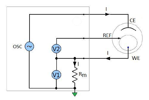
The unknown impedance of the working electrode is calculated from the measured voltage and current values (Fig. 2):
$$Z_\text{M} = \frac{V_2}{1}=\frac{V_2}{V_1}\, R_\text{m} \tag{1}$$

Potentiostat stray Capacitances

An instrument is made of real, hence imperfect components. At high frequency most of the artifacts come from the input stray capacitances. A model of the instrument is shown in Fig. 3, which includes the main stray capacitances: the counter to the reference capacitance, the reference to the ground capacitance, the reference to the working and the working to the ground capacitance.

Figure 3: Model of the potentiostat including the four main stray capacitances.

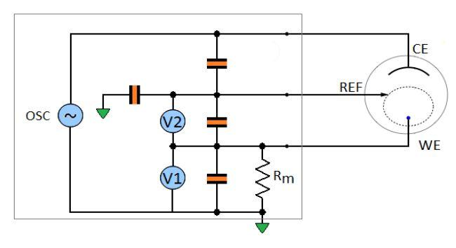
The influence of the stray capacitances of the reference to the working and of the working to the ground are cancelled by the calibration of the instrument at the factory. To calibrate the instrument, standard devices are connected at the end of the leads of the standard cable and the instrument is adjusted (through computation/data storage) so that it measures within the specified accuracy.

EIS Accuracy Plot

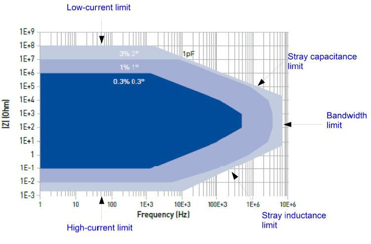
In Fig. 4, the shaded areas show different ranges of impedance that can be measured within a specified error in magnitude and in phase. Residual stray capacitances and stray inductances limit the measurement accuracy at high frequencies on high and low impedance cells, respectively. However, this accuracy plot is the highest accuracy one can obtain on standard devices. The electrochemical cell and its environment makes the real accuracy be not as good as the one in this plot. It is important then to understand the origin of the artifacts and to try to minimize them.

Figure 4: SP-200 contour plot.

EIS On Anelectrical Circuit

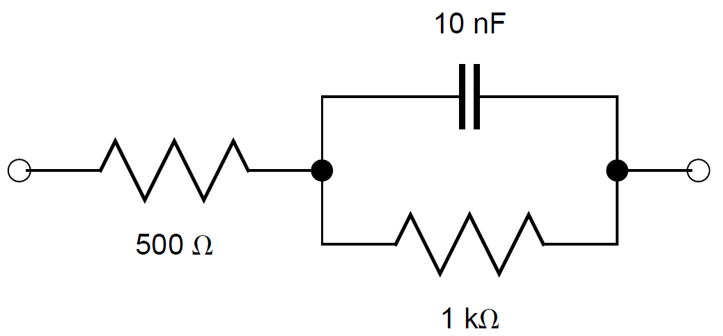
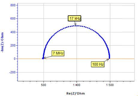
For the sake of simplicity, an electrical circuit in the middle range of the potentiostat impedance accuracy plot has been chosen. As expected, the impedance measurement performed with the SP-200 in the high frequency range from 7 MHz to 1 kHz corresponds to the effective impedance of the cell (Fig. 6).

Figure 5: Equivalent model of the potentiostat with simplified artifacts.

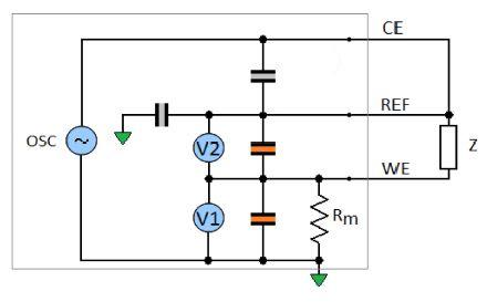
Figure 6: Electrical circuit in the middle range of the potentiostat impedance accuracy plot, corresponding Nyquist impedance diagram.

The same experiment is now performed with a 10 kΩ resistor mimicking a poor reference electrode (Fig. 7).

Figure 7: Model of the potentiostat with a simulated poor reference electrode.

The measured impedance (Figs. 6 and 8), represented in red in the Nyquist diagram is far from the previous measurement in blue. The equivalent measured impedance can be obtained from the Kirchhoff’s laws:

It can be noted that if R resistance is zero, the measured impedance Z_m equals the effective impedance Z given by (Fig. 6):

$$Z_\text{m}=\frac{Z(1+jωR_\text{m}C_2)(1+jωRC_4)-jωRR_\text{m}C_3}{1+ j \omega R(C_1+C_3+C_4)+j \omega R_\text{m}(C_2+jwRC_1C_3+j \omega RC_2(C_1+C_3+C_4))} \tag{2}$$

With r1 = 500 Ω, r2 = 1 kΩ and c2 = 10 nF.

$$Z = r_1 + \frac{r_2}{1+jωr_2c_2} \tag{3}$$

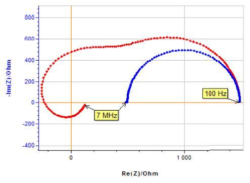
Figure 8: Measured impedance with poor reference electrode (red dots) and impedance diagram shown in Fig. 6 (blue dots).

Focus On The Reference Electrode

a. Model Fit
The Mathematica software was used to fit the measured data with the equation of Z_m (Eq. (1)).The plot obtained using the fit parameters (r1 = 500 Ω, r2 = 1.00 kΩ, c2 = 9.99 nF, R = 10.0 kΩ, C4 = 17.8 pF, Rm = 1.00 kΩ, C1 = 8.56 pF, C2 = 0.344 nF, C3 =52.0 pF), match pretty well the experimental data (Fig. 9). Also, the fit values of stray capacitances of the instrument are in good agreement with the expected values. Thus, we can say that the potentiostat model with artifacts we have proposed is most likely to be the correct one.

Figure 9: Measured impedance with poor reference electrode (red dots), impedance diagram shown in Fig 6 (blue dots) and fitted curve (green curve).

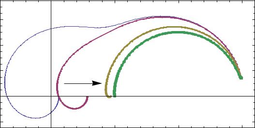
Generally, a platinum wire and a parallel bypass capacitor should be added to the reference electrode to overcome the EIS high frequency artifacts. BioLogic provides a special EISR-XR820 reference electrode model which includes a bypass 10 nF capacitor. This capacitor makes the reference electrode continue to provide a constant voltage reference while its impedance (reactance) decreases as the frequency increases. Why 10 nF ? The value of this capacitor could be higher but it would not change very much as 1 MHz impedance of a 10 nF capacitor is only 16 Ω. Figure 10 shows the change of Z_m with the C4 value. For the sake of simplicity we considered C4 as a reference bypass capacitor. Note that Z_m for C4 = 10nF.

Figure 10: Change of Nyquist diagram of Z_m with C4 value. C4/nF = 0:01; 0:1; 1; 10, from left to right.

b. Real electrochemist life

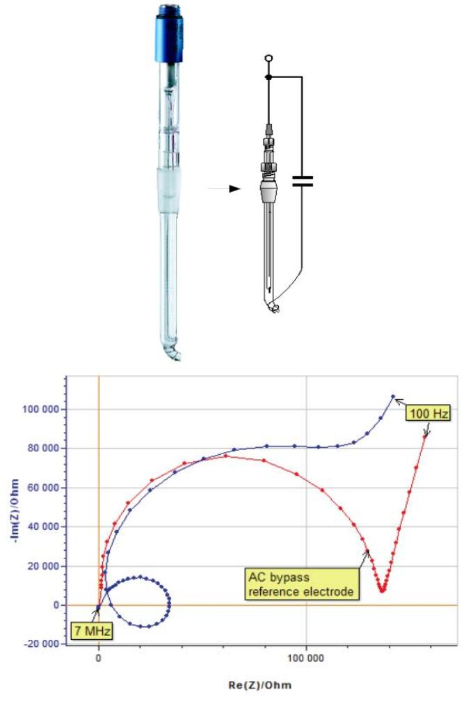
The impedance spectrum (Fig. 11) of a glassy carbon electrode in a ferrocene solution was measured with an R-XR300 Ag/AgCl reference electrode fitted with a bridge tube. An unexperimented user could even find a good fit with a non-realistic equivalent electric circuit.

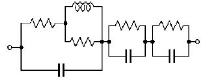
Figure 11: Impedance spectrum of a glassy carbon electrode in a ferrocene solution with a poor reference electrode and fit of the data using the circuit model.

The same experiment was carried out with the R-XR820 AC bypass reference electrode. The two plots move away from each other at relatively low frequency (Fig. 12).

References

1) Application note #5 “Precautions for good impedance measurements”
2) Keysight Impedance Measurement Handbook. 6thEdition (2016).
3) S. Chechirlian, P. Eichner, M. Keddam, H.Takenouti, H. Mazille, Electrochim. Acta., 35 (1990) 1125.
4) S. Fletcher, Electrochem. Com., 3 (2001)692.
5) A. Sadkowski, J.-P. Diard, Electrochim.Acta., 55 (2010) 1907.
Revised in 01/2020