Constant power technique and Ragone plot Battery & Electrochemistry – Application Note 6

The aim of this document is to describe the Constant Power (CPW) technique. This technique, available with EC-Lab^® software (since V8.10), is applied in a Li-ion battery test and is available with all Bio-Logic instruments.

The Constant Power technique has been designed to study the discharge (eventually the charge) of a battery or a cell (made of intercalation compounds) at successive constant power. The constant power control is made by holding the power (i.e. the factor E*I) to a constant value. During the discharge, the cell potential decreases. In order to hold a constant power, the current is adjusted and will increase. This can be shown on the following figure.

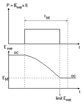
Figure 1: CPW discharge control (P) and measure (E_we) vs. Time.

The constant power technique is especially designed for battery testing. This technique is commonly used for Ragone plot representations (Power vs. energy) [1,2]. The usual protocol consists of successive sequences made with a:

• Discharge to P/2ⁿ watts with n the sequence number.
• Open circuit period after the discharge.

In this experiment, the cell has been previously fully charged in galvanostatic mode (C/5). P (= E·I) is chosen according to E at the beginning of the experiment and according to C (capacity of the cell). At the beginning of the experiment, the cell is charged so that E = 4.2 V. The power chosen for the first constant power step is 8 W. Then the current at the beginning of the experiment is less than 2 A in absolute (2C).

Note:

1. The user must be conscious that the current in discharge mode is negative.
2. The final current will be greater (in absolute) than the current at the beginning of the experiment.
3. It is necessary to use a power booster to deliver the desired current. Each channel board can deliver 400 mA continuous.

The first step is limited with a minimum potential for the cell (3 V). The final current is then 2.7 A. The user must choose the booster according to the final current of the first power step. Between each of the constant power steps, an OCV period allows the electrochemical system to equilibrate. This OCV period is limited by a minimum potential variation versus time. Each of the constant power steps can be seen in the protocol table. The duration of each step has been chosen in order to not be the limiting factor (that is E_M = 3 V). It is the same for the OCV period.

The following figure (Figure 2) shows the change of versus energy.current and potential during the CPW experiment

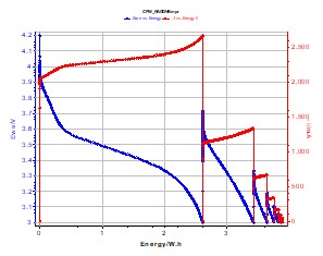
Figure 2: E measured (in blue) and –I adjusted (in red) change vs. Energy during a CPW experiment on a Li-ion battery (1.35 A·h). P = 8 W.

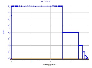
Figure 3: Power vs. energy plot for a Li-ion cell (1.35 A·h). P = 8 W.

One can see that for a constant power discharge, the positive electrode potential decreases, and the current decreases in the negative direction but it increases in absolute to compensate the potential fall. In Figure 2, the current (red line)  has been represented in absolute form in order to see the simultaneous evolution of E and I. E and I variation for constant energy values are obtained during OCV periods.

The plotted current values are absolute values (negative in reality). In order to have a constant power, the working electrode potential decreases when the current increases (in absolute).

The power vs. energy plot for a Li-ion (1.35 A·h) battery is presented on Figure 3. Each constant power is separated with an OCV period limited with a potential variation dE_R/dt = 2 mV/h.

A process called “Constant Power protocol summary” has been especially designed for Ragone plot representations. To use this data process, click on “process” in the graphic window or choose “Process data\Constant Power protocol summary” in the File menu. Then the processing window (Figure 4) appears.

This process window is made of a table containing the characteristic variables of each power step, such as the time, the energy, and the charge of the end of the step; the working electrode potential; and the current that crossed the cell at the beginning and the end of the step. The “Copy” tab allows the user to paste the values of the table in graphic software in order to have a Ragone plot (see Figure 4).

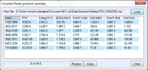
Figure 4: CPW process window.

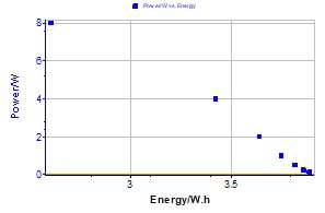
Figure 5: Ragone plot for a Li-ion cell (1.35 A·h).

The data points of the Ragone plot can be inserted in a domain defining the cell characteristics and material. The batteries are classified in this representation according to their power and energy properties.

References

- M. Conte, P.P. Prosini, S. Passerini, Mat. Sci. and Eng. B108, (2004) 2.
- T. Christen, M.W. Carlen, J. Power Sources, 91, (2000) 210.
Revised in 07/2018