Introducing the Microscopic Image Rapid Analysis (MIRA) software Scanning Probes – Application Note 5

Introduction

MIRA software is an optional representation and analysis software that is developed by Prof. Gunther Wittstock [1-5], based at the University of Oldenburg. The software offers a full range of graphical representations specially designed for line and area map data. One of the most interesting features is the ability to fit Scanning Electrochemical Microscopy (SECM) approach curves, giving access to various physical and chemical parameters related to the experiment itself. This note introduces some of the features of the MIRA software, with a special focus on the SECM approach curves fitting tool.

Plotting Data Obtained with M370 Or M470

Opening files in MIRA

The native files obtained from the M470, M370, or SECM150 software (referred to collectively as the SCAN-Lab software) can be opened with the latest versions of MIRA. If using a MIRA release from before 15 March 2021, please see Appendix 1.

All file types produced by the SCAN-Lab software are compatible with MIRA. This includes the area maps of all techniques including all the different data available in dc-, ac- and ic-SECM, as well as approach curves obtained with dc- and ac-SECM, and Cyclic Voltammograms (CV).

MIRA software contains tools that have been developed by Prof. Wittstock and default tools written and provided by IDL (Interactive Data Language v.8.1 by Research Systems Inc., Boulder Colorado). These imaging tools have a name which usually starts with an i.

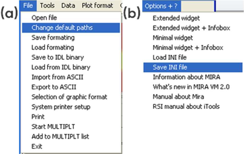
When starting the MIRA software, the window seen in Fig. 1 pops up, displaying which .ini files are available. .ini files define the folder that will be opened by default, the default output folder as well as the default representation. The default paths can be changed as shown in Fig. 2a and these changes can be saved in a new .ini file as shown in Fig. 2b. Note: .ini files are located in MIRA\startup.

Figure 1: Configuration window showing the available .ini files.

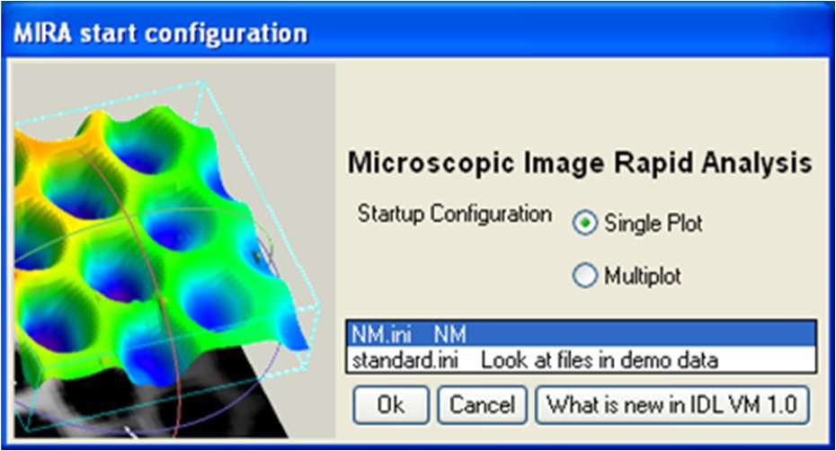
Figure 2: (a) Changing the default paths, (b) saving the new .ini file.

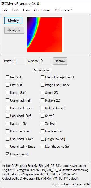
When opening a file, the window shown in Fig. 3 will appear. It shows the default representation of the opened data in a small window and all the available representations. The representation option to be selected depends on whether an area scan, or line plots (e.g. approach curves or CVs) has been loaded. This will be covered in the following sections.

Figure 3: The main window of MIRA.

Area Scans

MIRA is compatible with area scans produced by any of the techniques available in the SCAN-Lab software. Throughout this section the figures are produced from the SECM area scan demo data provided with MIRA (…MIRA_VM_02_64\demo\DEVICES\Biologic_full\SECMAreaScan.uas).

After opening an area scan in MIRA it is possible to display the data using a number of representation options. Representations which provide a 3D projection of the data are:

• Net Surf.
• Line Surf.
• Illumin. Surf.
• User-shad. Net
• User-shad. Lines
• User-shad. Surf.
• Illumin. + Net
• Illumin. + Lines
• User-shad. + Net
• User-shad. + Lines

Any “Net” representation includes a wire frame of the data, while “Line” representations include lines in the x axis only. “Illumin.” and “User-shad.” representations include a color scale.

2D projections are produced if any of the following options are selected:

• Image Height
• Interpol. Image Height
• Image User Shade
• Contour
• Image + Cont.
• [Height no Scl]
• [User Shade no Scl]

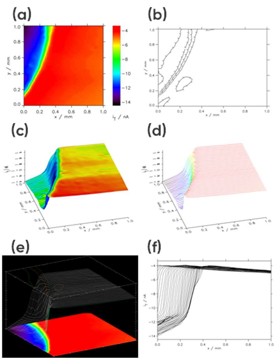
When “Show3” is selected the resulting plot will include a 2D projection, 3D projection, and contour plot, Fig 4e. Finally, if “Multiple 2D” is selected the X line data making up the area scan will be overlaid as a line scan, Fig. 4f.

Once the plot type, or types are selected, clicking on the “Redraw” button opens a new window showing the data. Examples of data plots are shown in Fig. 4.

Figure 4: Example area scan representations: (a) Interpolated Image Height, (b) Contour, (c) User Shade + Lines, (d) User Shade Lines, (e) Show3, and (f) Multiple 2D.

The plotted data can also be saved as a graphical file using the “Print” command in Fig. 2a.

The parameters of the export can be changed using the “Selection of graphic format” also shown in Fig. 2a. The file will be exported into the default folder. It can be saved in various matric formats (.jpeg, .tiff, .bmp) as well as vector formats (.ps, .eps).

The palette used to plot the data can be changed using the following command Tools->XLoadct.

Line Plots

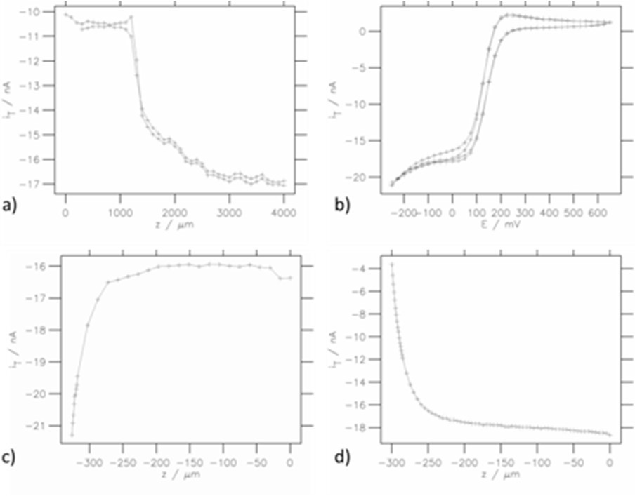
The MIRA software is also compatible with any line plot produced by the SCAN-Lab software such as line scans, CVs and approach curves. Line plots are loaded into MIRA in the same way as area scans. This data is plotted by selection of the “Single 2D” option. Examples are shown in Fig. 5.

Figure 5: Various line plot representations: a) SECM forward-backward line scans, b) CVs, c) Approach curve on conducting region, d) Approach curve on insulating region.

Using the fitting tool

One of the most interesting tools of MIRA is the ability to fit dc-SECM approach curves and have access to experimental parameters and reaction kinetics.

The Curve fitting tool is accessible using the Analysis button on the left of the data display window, Fig. 6.

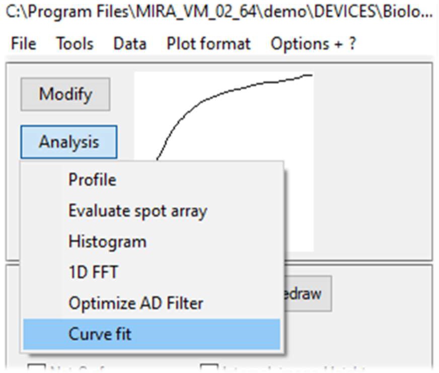
Figure 6: Analysis menu options to access SECM approach curve fit window.

In the next window, all of the conditions required to fit the approach curve are displayed, this includes the analytical expression used to fit the data, the fitting parameters and the paper in which it was first described, Fig. 7.

Figure 7: Fitting parameters available in the approach curve fitting window.

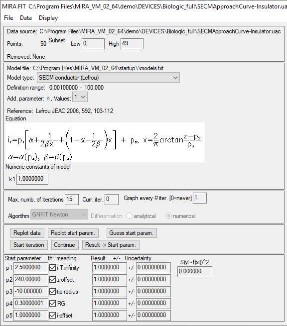
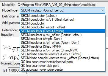
In this document, the insulator approach curve located in the MIRA demo folder (…MIRA_VM_02_64\demo\DEVICES\Biologic_full\SECMApproachCurve-Insulator.uac) is fit. In this experiment an approach has been performed to an insulating sample. The probe position is at first 0 and then approaches the sample, resulting in negative values of z. To fit the approach curve the equation “SECM insulator w/o i_offset (Cornut, Lefrou)” was used [6], Fig. 8.

Figure 8: The choice of equations available to fit the approach curves.

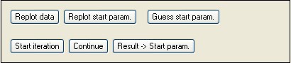
After choosing the equation corresponding to user-specific conditions (approached material, current offset, etc.), the initial parameters are determined by clicking on “Guess start parameters” in the fitting commands window, and then “Start iteration”, Fig. 9. “Guess start parameters” uses an algorithm, to analyze the curve and find starting values which are close to the final values.

Figure 9: The fitting commands window.

Clicking on “Guess Start Parameters” and then “Start iteration” with 30 iterations leads to the results shown in Fig. 10.

Figure 10: The results window obtained with “SECM insulator w/o i_offset (Cornut, Lefrou)” expression. In red the curve obtained using the Start parameters, in green the curve obtained after fitting.

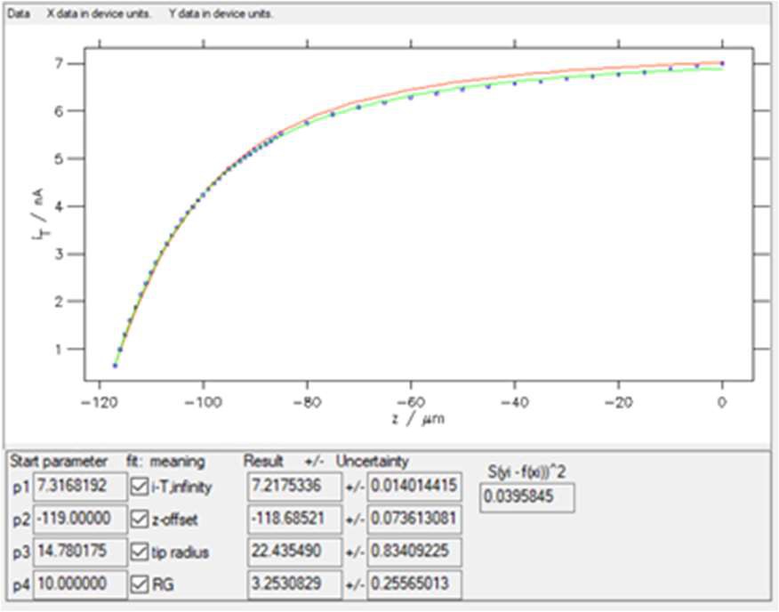
Four parameters are obtained when fitting an approach curve:

• i-T, infinity is the current when the probe is in the bulk or at an infinite distance from the sample.
• z-offset is the opposite value of the distance between the probe

and the sample at the beginning of the approach.

• tip radius is the radius of the active region of the probe, e.g. the Pt disc.
• RG is the ratio between the diameter of the glass sheath around the metallic electrode and the diameter of the active region, e.g. the Pt disc. For further information on the use of MIRA to determine the RG ratio of the probe please see TN#11 [8].

The starting values and the values after fitting are shown along with their error, as well as the residuals and the square of the sum of these residuals, also called the χ² parameter (considering the variance is equal to 1, as there is only one experiment done). This function χ² is used in the minimization process, which is based on the Gauss-Newton algorithm [7]. The lower this number, the better the fit (for the same number of points). In the example shown in Fig. 10, χ² ≈ 0.039.

There are two ways to improve the fit of the approach curve. The first option is to continue the fit from the last run, this is possible by clicking on “Continue”. The second option is to remove bad points at the start of the experiment, when the probe is far from the surface, which are less well fit than those when the probe is near the surface. To do this the top left of the window, Fig. 11, is used.

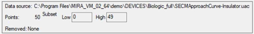
Figure 11: Data removal window.

Entering 5 in the “Low” box will remove the first five points in the lower values of the variable (z). Then click on the “Replot data” button shown in Fig. 9. The results of the fitting done on these new data are shown in Fig. 12.

Figure 12: Fitting results obtained on the newer dataset obtained with “SECM insulator w/o i_offset (Cornut, Lefrou)” expression.

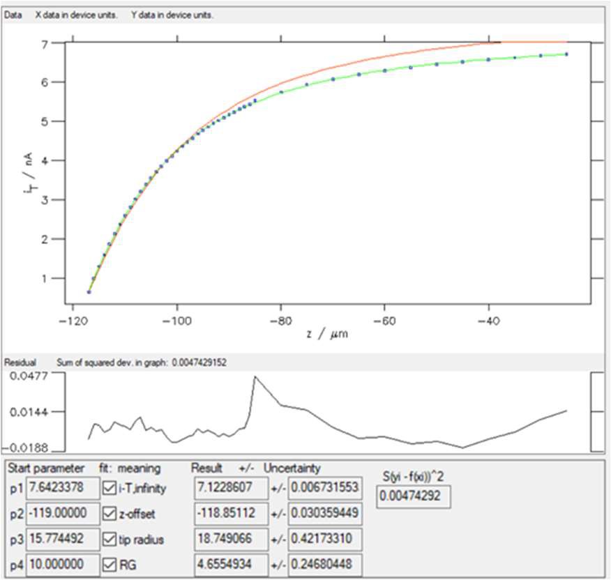
Now, the χ² ≈ 0.005, which is expected as the number of points has been reduced but also means that the fit is of better quality.

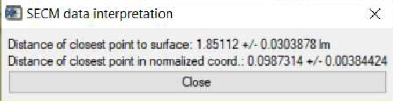
Further to the information available in the main curve fit window, once an approach curve has been fit, users can also determine the point of nearest approach in the curve, i.e. how far the final point in the approach curve is from the sample surface. Following the fitting, this is then accessed through the SECM data interpretation option accessible through the Display menu. Using the approach curve as fit in Fig. 12, the point closest to the surface is seen to be (1.85 ± 0.03) µm from the surface, Fig, 13.

Figure 13: The SECM data interpretation option of the curve fitting tool is used to display the distance of closest approach to the surface.

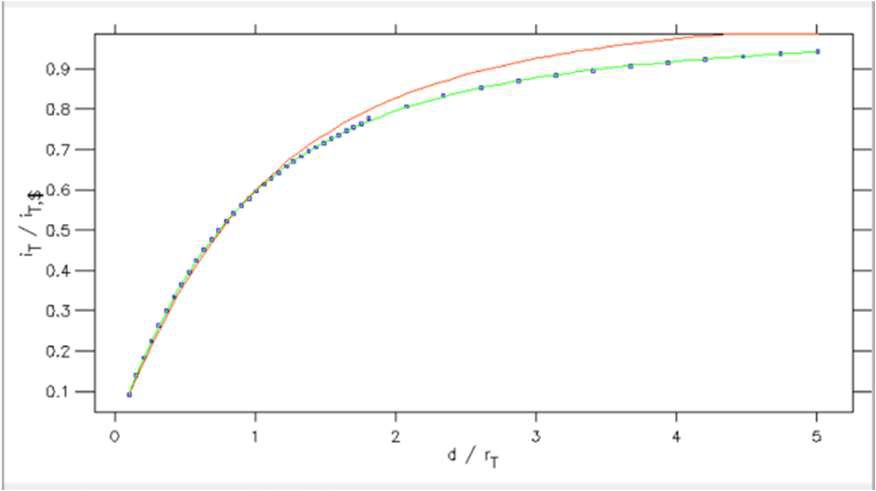
From within the Curve fitting tool it is also possible to plot the SECM approach curve on normalized coordinates. This is possible using the Plot normalization option in the Display menu. Using this tool, Fig. 14, users can plot against a normalized x or y axis, or both. In Fig. 15 its use is demonstrated for the approach curve from Fig. 12 plotted against a normalized x and y axis.

Figure 14: Plot normalization window.

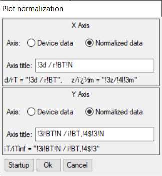
Figure 15: SECM approach curve plotted against normalized distance (x) and current (y) coordinates.

Tips

1. In the approach curve shown above, the step size was initially 5 µm and the scan speed 10 µm/s, when the probe was near the surface the step size was reduced to 1 µm and the scan speed 2 µm/s. It is recommended to perform approach curves with a step size smaller than 1 µm and a scan speed of 1 µm/s or less. With these conditions, the experimental values do not diverge too much from the theory and the trueness of the fitting will be increased (and the χ² factor decreased).
2. Using parameters independently determined can be beneficial for the fit. For example, the value of the tip radius can be determined by cyclic voltammetry and entered in Fig. 10 in the “Start parameter” box. Then, if the box under “meaning” is unchecked, the parameter will not be considered in the fitting process.

References

- 1. G. Wittstock, T. Asmus, T. Wilhelm, Fresenius’ Journal of Analytical Chemistry, 367 (2000) 346–351
- U. M. Tefashe, K. Nonomura, N. Vlachopoulos, A. Hagfeldt, G. Wittstock, Journal of Physical Chemistry C, 116 (2012) 4316-4323.
- C. Nunes Kirchner, M. Träuble, G. Wittstock, Analytical Chemistry, 82 (2010) 2626-2635
- W. Nogala, M. Burchardt, M. Opallo, J. Rogalski, G. Wittstock, Bioelectrochemistry, 72 (2008) 174-182
- G. Wittstock, M. Burchardt, S. E. Pust, Y. Shen, C. Zhao, Angewandte Chemie International Edition, 46 (2007) 1584–1617
- R. Cornut, C. Lefrou, Journal of Electroanalytical Chemistry, 608 (2007) 59-66
- K. Ebert, H. Ederer, Computeranwendungen in der Chemie. 2. Ed., VCH, Weinheim 1985, S.323.
- SCAN-Lab Technical Note #11 “Determining the probe diameter and RG ratio in an SECM experiment”
Revised 07/2023