Dynamic resistance determination. A relation between AC and DC measurements? EIS & Battery – Application Note 38

Introduction

Currently, several types of batteries are being investigated (Li-ion, LiFePO₄, etc). Each type has its own specification such as nominal voltage (V), capacity (Ah), power (W), energy (Wh), cyclability. The apparent resistance R_Δt of the battery is also a relevant parameter.

This resistance can be determined by a simple current interrupt technique. In this technique, a current pulse is applied to the battery and the voltage shift is measured after a certain period of time Δt (Fig. 1). The ratio of the voltage shift ΔE and the current difference ΔI yields to a resistance, R:

$$R_{\Delta t}=\frac{\Delta E}{\Delta I}=\frac{E_2-E_1}{I_2-I_1} \tag{1}$$

The duration Δt may be different depending on the procedure used. For example, this period is 30 s in the procedure of the United States Advanced Battery Consortium (USABC) [1].

Figure 1: Current and voltage change versus time after current pulse applied at t₁.

This apparent resistance is called dynamic resistance when it is measured while the device is in operation [2-4]. For a battery, this value depends on the Δt, ΔI, Depth-Of-Discharge (DOD), State-Of-Charge (SOC), State-Of-Health (SOH)…

In this application note, we will show how to determine the dynamic resistance with a DC technique. In the second part, the relationship between the dynamic resistance and impedance will be discussed. During the discharge, the dynamic resistance and the impedance are determined by DC measurement or by AC measurement (Electrochemical Impedance Spectroscopy; EIS), respectively.

Experimental

The measurements discussed hereafter were carried out on a LiFePO₄ battery with capacity of 3.2 Ah (initially charged).
EC-Lab^® software is used to monitor a VSP, equipped with a 4A internal booster. EC-Lab^® is also used to process the resulting data.

Dynamic resistance determination

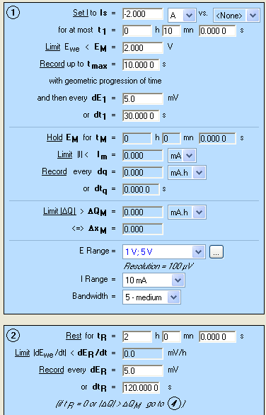
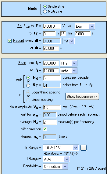
As described above, in order to determine the dynamic resistance of the battery, a galvanostatic pulse has to be applied to the battery. As the voltage change does not follow a linear evolution (Fig. 1), a sampling rate with geometric progression is of interest. GCPL5 technique offers this sampling rate with a common ratio of 2 during t_max. All the other parameters of the GCPL5 technique are similar to the GCPL technique which is shown in a previous application note [5]. A discharge of 2 A is applied to the cell and the dynamic resistance determination is performed periodically. The settings of GCPL5 are displayed in Fig. 2.

Figure 2: GCPL5 settings.

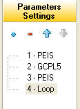
To complete the dynamic resistance determination, an EIS measurement is done after each sequence of discharge. The setting of the experiment, which is a series of linked techniques, is shown in Fig. 3. EIS measurements are indicated by the green arrows in Fig. 4. (see next paragraph).

Figure 3: GCPL5 and EIS linked techniques.

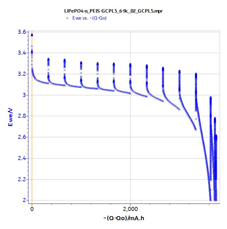
A typical behavior of the LiFePO₄ battery is observed (Fig. 4) i.e. a slow voltage decreases down to the capacity of the cell and then a deep voltage drop.

Figure 4: GCPL5 data.

The resulting data are processed via the “Process Data” window.  For Dynamic resistance determination, “Keep only values with geometric progression of time” and “Rapp” (dynamic resistance) boxes have to be ticked (Fig. 5) (uncheck “Allow reprocessing” box).

Figure 5: Dynamic resistance process.

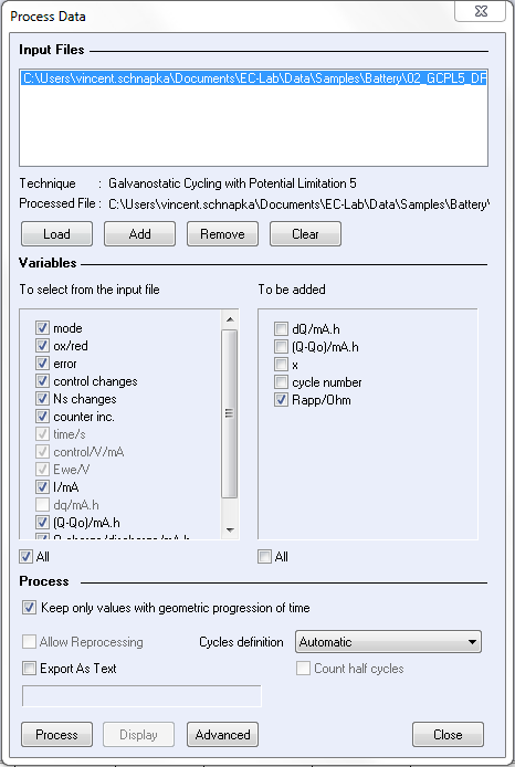
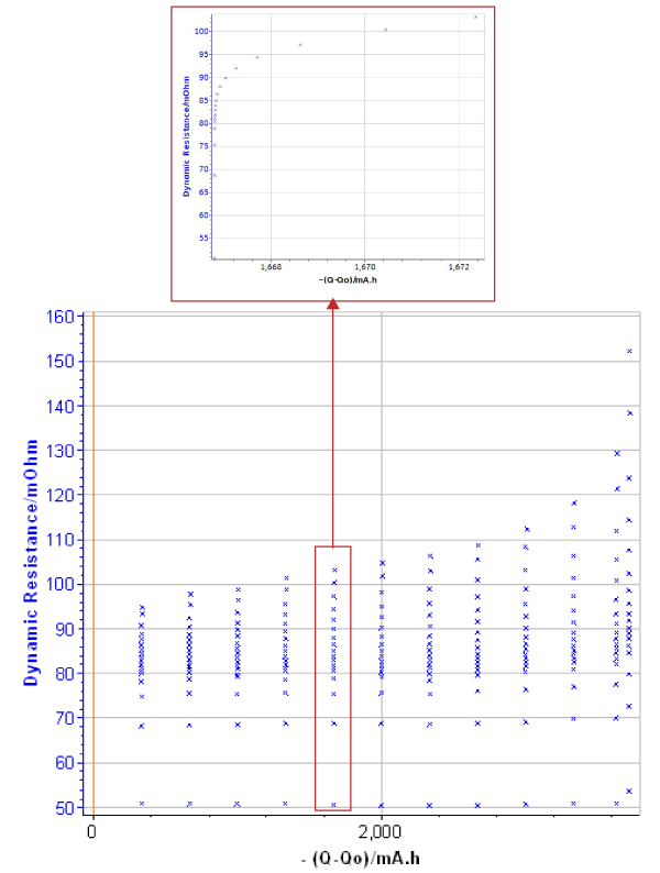
Figure 6 shows that the dynamic resistance increases when the battery is discharged. Data resulting from GCPL investigation can be processed and it is possible to determine the dynamic resistance for several Δt (Fig. 6B).

Figure 6: Dynamic resistance change. A) during the whole discharge (inset: zoom of the 6th discharge step); B) at certain period after the pulse: 200 µs, 1 ms, 1.6 s and 10 s.

EIS measurement

To complete the characterization, EIS investigations are performed after each pulse. The settings are shown in Figs. 2 and 7.

As the voltage of the cell changes during the measurement, it is recommended to activate the patented “drift correction” [6].

Figure 7: Setting of the experiment

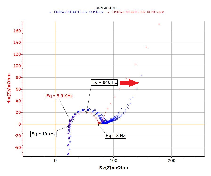
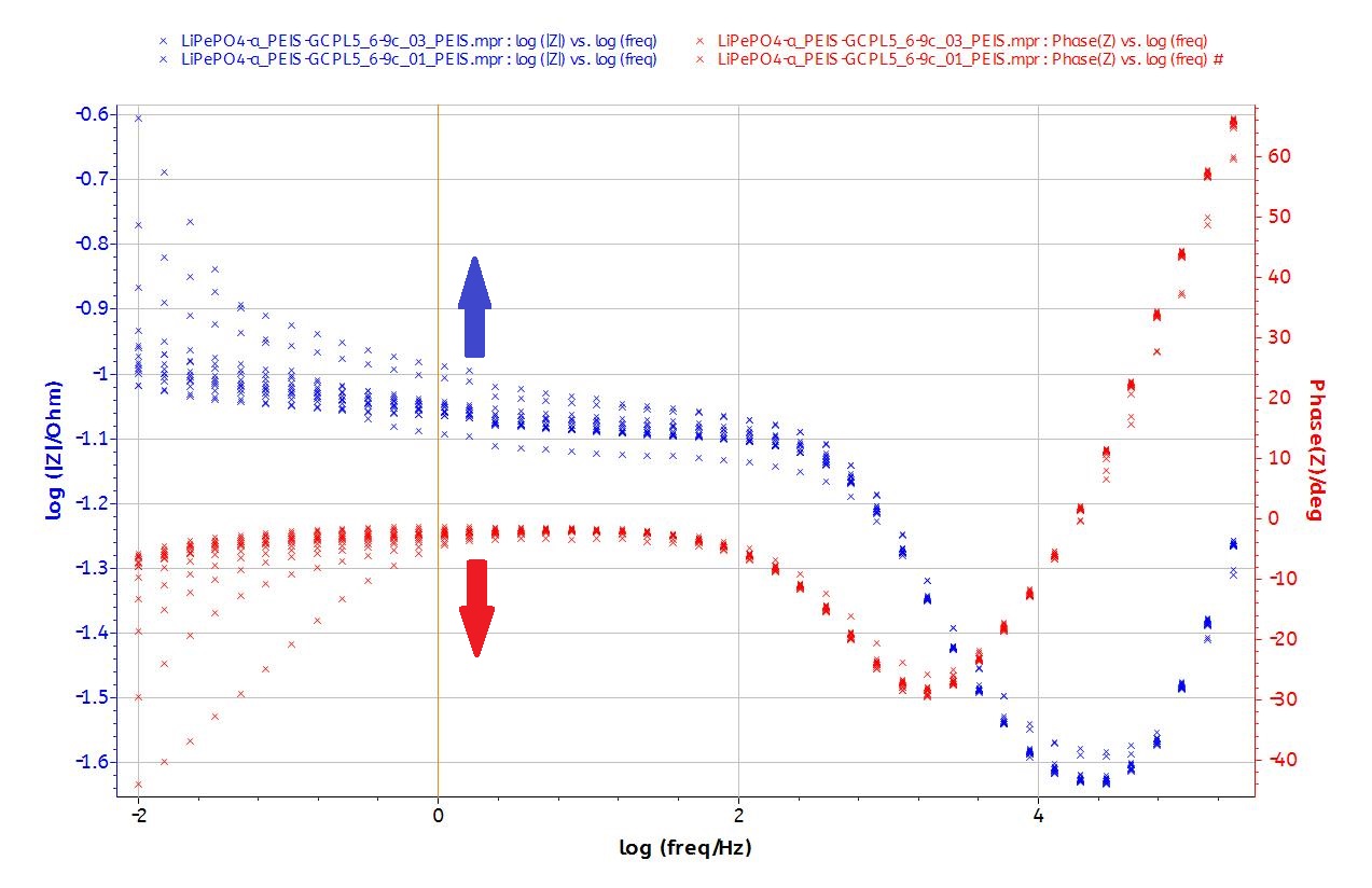
The EIS plots (Fig. 8) show the typical behavior of the LiFePO₄ battery (display one semicircle at intermediary frequencies, a diffusion behavior at low frequencies and inductance behavior at high frequencies).

Figure 8: Nyquist and Bode plots of the EIS data.

DC/AC data comparison

The DC (time domain) and AC (frequency domain) data are compared at two levels. Firstly (part V-1), the dynamic resistance resulting from GCPL investigation is compared to the resistance fit from the EIS data. Secondly (part V-2), the step response (i.e. the response of the system to a discrete potential step) of the system is calculated from GCPL data at several Δt (not only one point as it was done in the first part) and compared to the EIS data.

One point comparison

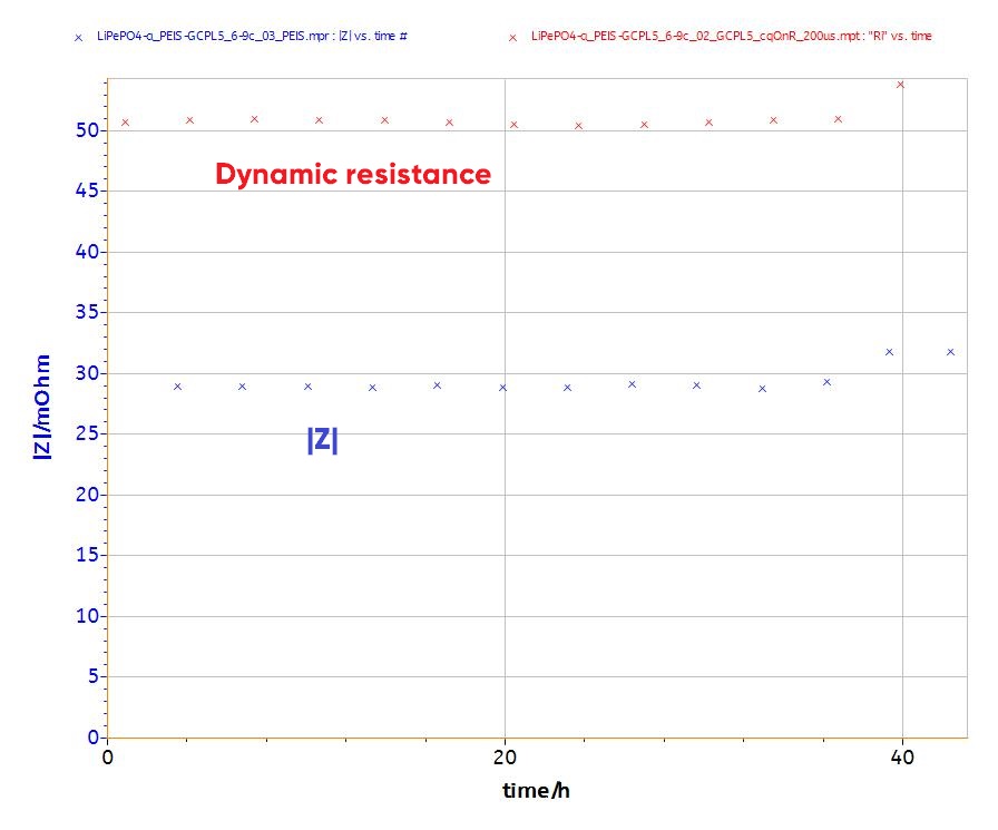
To compare the data between DC and AC experiments, the dynamic resistance and impedance after each discharge step are plotted versus time (Fig. 9). Both DC and AC data have to be given in terms of frequency. The DC data conversion is done by the relationship (2).

$$\omega=\frac{1}{\Delta t} \tag{2}$$

where is the pulsation in rad s^-1.

So, if Δt of 200 µs is considered, the corresponding frequency is 5 kHz.

Figure 9 shows that both dynamic resistance (DC measurement) and impedance (AC measurement) yield to similar trends (small increase) and have the same magnitude (between 25-50 mΩ).

It is noteworthy that the impedance is not a pure resistance at 5 kHz (Fig. 8). The phase at this frequency is -20°.

Figure 9: Dynamic resistance and impedance plots resulting from DC (200 µs) and AC (~5 kHz) investigations, respectively.

Step response calculation on the whole frequency range

In order to compare the time domain and the frequency domain measurement, it is possible to calculate the step response of the battery using the inverse of the Laplace Transform (L^– 1).

For example, let us consider the equivalent circuit R1 + L1 + R2/C2 + W1 (typical for a battery):

The impedance is given by:

$$Z\left(s\right)=R1+L1s+\frac{R2}{1+R2C2s}+\frac{\sigma}{\sqrt s} \tag{3}$$

For a step of current, , the step response of the circuit is given by:

$$E\left(t\right)=L^{-1}\left[\frac{\delta I}{s}Z\left(s\right)\right]\ = \delta I(R1+L1 \delta(t))+ R2\left(1-exp{\left(-\frac{t}{R2C2}\right)} + \frac{2\sigma\sqrt t}{\sqrt\pi}\right) \tag{4}$$

Where δ(t) is the Dirac delta function.

The ratio E(t)/I(t) and modulus are given by the equation (4) and (5), respectively.

$$\left|Z(\omega)\right|= \left(\left(R1+ \frac{\sigma}{\sqrt{\omega}}+ \frac{R2}{1+R2^2C2^2 \omega^2}\right)^2 + \left(R1+ \frac{\sigma}{\sqrt{\omega}}+ \frac{R2}{1+R2^2C2^2 \omega^2}\right)^2 \right)^{\frac{1}{2}}\\ = \sqrt{2}\left(R1+ \frac{\sigma}{\sqrt{\omega}}+ \frac{R2}{1+R2^2C2^2 \omega^2}\right) \tag{5}$$

Modulus versus angular frequency (from AC measurement) and ratio E(t)/I(t) versus the inverse of Δt (from DC measurement) are plotted in Fig. 10. The superimposition of both plots show that data coming from AC and DC measurement are in good agreement.

Figure 10: Dynamic resistance (DC simulation) and Z plot versus logarithm of Δt or 𝝎, respectively (bottom). For information, the corresponding Nyquist plot is given at the top.

References

1) Electric Vehicle Battery Test Procedures Manual, Rev2 (1996) Appendix I.
2) M. Safari, C. Delacourt, Journal of the Electrochemical Society, 158(10) (2011) A1123.
3) K. Taken, M. Ichimura, K. Takano, J. Yamaki, S. Okada, Journal of Power Sources 128 (2004) 67.
4) A. Tenno, R. Tenno, R. Suntio, IEEE (2002) 176.
5) Application Note #5 “Protocols for studying intercalation electrodes materials: Part I: Galvanostatic cycling with potential limitation (GCPL)”
6) Application Note #17 “Drift correction in electrochemical impedance measurements”
Revised in 08/2019