

How to check and correct non-stationary EIS measurements using EC-Lab® (part 1) Corrosion – Application Note 69-1
Latest updated: June 4, 2024Abstract
This application note presents the various tools available in EC-Lab® that can be used to check and correct the non-stationarity of your EIS measurements. Using galvano control, the proprietary Non-Stationary Distorsion indicator, and the instantaneous impedance analysis tool Z Inst, users can ensure that EIS measurements are correctly interpreted and fitted. This application note shows the use of such tools on data obtained on a corroding electrode.
Introduction
For valid Electrochemical Impedance Spectroscopy (EIS) measurements, the system under investigation should be linear, stable, causal and stationary [1,2]. In this note, the term “stationarity” comprises steady-state and time-invariance.
Steady-state is the state of a system after its transient state. For example, an R/C circuit submitted to a potential or current step is in a transient state and sees its response change until a certain amount of time has passed.
Time-variance refers to a system whose parameters defining its transfer function change with time. As an example, a corroding electrode whose polarization resistance is changes over time, either because of corrosion or of passivation, is a time-variant system.
The two properties may be difficult to separate.
The most classical use of EIS in corrosion is for the determination of the polarization resistance Rp using the Stern or Wagner-Traud relationship [3-7]. A corroding system is a non-stationary system specifically after the first instant of immersion. The change in parameters can greatly affect the impedance data especially at lower frequencies [8].
In this first part of application note 69, we will present various tools implemented in EC-Lab® to help check and correct the time-variance of measurements. These tools will be applied to measurements on a corroding mild steel electrode. The second part will apply these tools to a discharging battery [9].
Experimental conditions
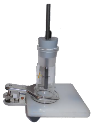
Potentio-controlled EIS measurements (PEIS) were performed on a mild steel sample (undisclosed composition) using a coating cell (Fig. 1), a carbon rod electrode, an Ag/AgCl reference electrode and a 0.1 M H2SO4 solution (EL-COAT).

Figure 1: Coating cell with a carbon rod counter electrode and an Ag/AgCl reference electrode.
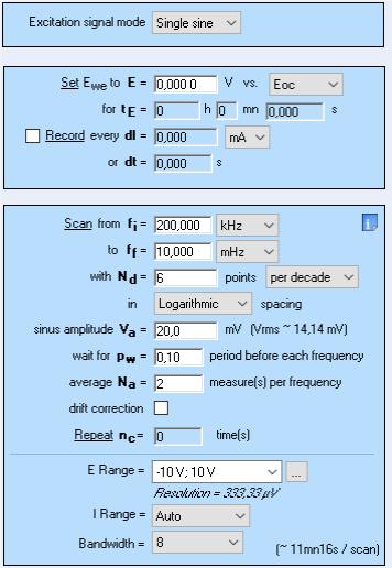
Six EIS successive measurements were performed using a BioLogic SP-200 potentiostat/galvanostat, EC-Lab® software and the parameters shown in Fig. 2.

Figure 2: PEIS parameters used for the EIS experiments on a mild steel sample undergoing general corrosion.
Results
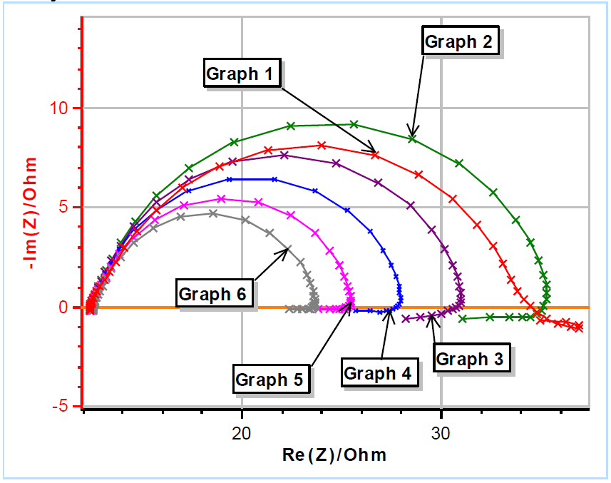
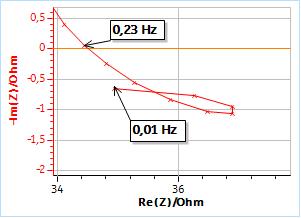
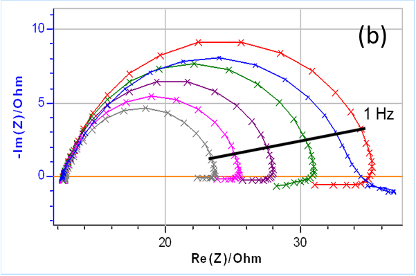
The results are shown in Fig. 3. Please note that the frequency sweep was performed from high to low values. It can be seen in Fig. 3a that right after immersion (Graph 1 in Fig. 3a), the instantaneous polarization resistance seems to increase and then to rapidly decrease, hence the occurrence of a loop at lower frequencies (Fig. 3b).
The next five impedance diagrams show the “fold-over” of the values at lower frequencies, which seems to be characteristic of a decrease of the instantaneous polarization resistance. It should be noted that the measured data show an inductive behavior at lower frequencies, with values that have a positive imaginary part.
We can assume, considering the pH of the electrolyte, that the metal corrosion is driven by the Volmer-Heyrovský mechanism: this is a common two-step mechanism for hydrogen evolution, with an adsorption step and dihydrogen release step. It was calculated that the impedance of such a reaction shows an inductive loop at lower frequencies [10]. It was shown that these experimental data correspond very well with simulated impedance data where the polarization resistance increases or decreases with time. More details can be found in [11,12].
a)
b)
Figure 3: (a) Nyquist representation of the impedance data (200 kHz – 10 mHz frequency range) obtained on a mild steel sample (undisclosed composition) just after immersion in 0.1 M H2SO4. The six measurements were successively performed. (b) Close-up on the low frequency part.
Which data can be reliably interpreted and considered as valid? How can it be made sure that the data interpretation is not erroneous, for example that the time-variance effect is not interpreted as an inductive loop ? In the next part of this paper, we will present the tools available in EC-Lab® that can help address such problems.
How to check and correct time-variance using EC-Lab®
Perform EIS with galvano control
Impedance spectroscopy can be performed by controlling the potential, which means that the input signal is a potential modulation around a DC potential and the response of the system is a current modulation around a DC current. In this case, the transfer function is not the impedance but the admittance of the system.
However, the input modulation can also be an AC current modulation around a DC current, in which case the response is an AC potential modulation around a DC potential. In this case, the transfer function is the impedance of the system. In EC-Lab® this technique is called GEIS.
The impedance diagrams shown in Fig. 3a were obtained using Potential-controlled EIS (PEIS). Figure 4 shows the evolution of the DC current during this experiment, for which the potential modulation is applied around the Open Circuit Potential (OCP) measured just before the beginning of the PEIS.

Figure 4: Evolution of the DC potential and the DC current during the six potentio-controlled EIS experiments shown in Fig. 3a.
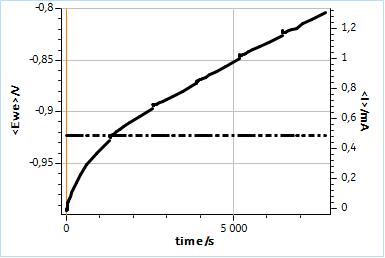
It can be seen in Fig. 4, that the potential is maintained at a constant level over the whole experiment duration but that the DC current moves away rapidly from zero, meaning that as time goes by, the sample is anodically polarized due to the evolution of its free corrosion potential (or OCP).
This phenomenon is illustrated in Fig. 5a, which shows that if the steady-state $I$ vs. $E$ characteristic of a corroding sample moves towards more cathodic potentials, the initial OCP becomes an anodic potential. Potentio-Controlled (PC) impedance measurements are not performed around the initial OCP but around a specific operating point on the anodic part of the steady-state curve.
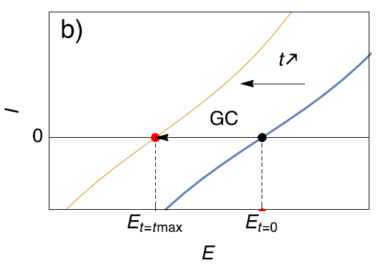
On the contrary, as illustrated in Fig. 5b, if impedance measurements are performed using current control (or Galvano-Control GC) and around zero current (which is equivalent to OCP), even though the steady-state curve changes and moves towards cathodic potentials, the modulation is still performed around the same point on the steady-state curve. To understand more about PEIS and GEIS, please see the corresponding application note [13].
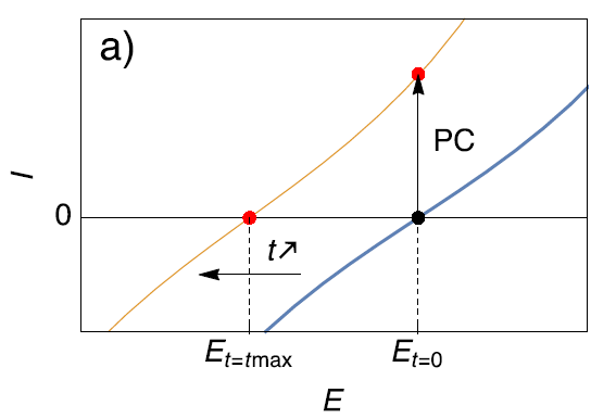

Figure 5: Description of the effect of (a) Potential Control (PC) and (b) Galvano control (GC) when the steady-state curve of the system is moving towards more cathodic potentials.
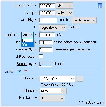
It is also important to note that the main drawback of the GEIS technique is the choice of input amplitude. While it is easy to choose a potential amplitude (generally tens of mV are good values to start), choosing a current input amplitude is not intuitive. In EC-Lab®, it is possible to use GEIS and a potential amplitude as can be seen in Fig. 6.

Figure 6: How to set a GEIS experiment with a potential input amplitude, also called GEIS-AA.
Non-Stationary Distortion (NSD) indicator
In this paper, as explained in the introduction, what we mean by non-stationarity is two-fold:
- The fact that the system is in a transient regime, that it has not yet reached its steady-state. Its transfer function stays the same throughout the experiment but its steady-state response is not reached instantaneously, it is lagging.
- The fact that the system sees its transfer function or the values of the parameters constituting its transfer function change over time. This is what we called throughout the paper time-variance.
Both phenomena have a specific effect on the response signal, which can be seen on the impedance diagram, but also on its Fourier Transform (FT), which gives a frequency representation of the signal. The FT of the time response signal of a stationary (and linear) system will show a line at the same frequency as the input signal. The response of a non-stationary system, whether it is in a transient state or time-variant will show lines which are not only at the same frequency as the input signal but also at adjacent frequencies.
The amplitude of the adjacent lines around the signal response at the fundamental frequency depends on the extent of the non-stationarity of the system.
We can introduce an indicator that can be used to quantify the non-stationarity of the signal, whether it is due to a transient state or to a time-variance. We call this indicator NSD. It is calculated as follows:
$$\text{NSD}(f)=\frac{1}{Y_f}\sqrt{Y_{f-\Delta f}^2+Y_{f+\Delta f}^2}\tag{1}$$
where $Y_f$ is the amplitude at the stimulation or fundamental frequency $f$, $Y_{f-\Delta f}$ and $Y_{f+\Delta f}$ are the amplitudes at the frequencies adjacent to the fundamental $f-\Delta f$ and $f+\Delta f$ and $\Delta f$ is the spectral frequency resolution.
All this is illustrated and explained in more details in the corresponding BioLogic white paper [14].
Please also note that the “drift correction” tool, shown in Fig. 6, can be used to account for and correct the non-stationarity of the system [15].
Figure 7a shows the NSD for the impedance measurements shown in Figs. 3, shown again here in Fig. 7b.
The NSD is dependent on the frequency. If the measurement is fast enough, it is not affected by the non-stationarity, especially by the time-variance of the system.
A NSD value as low as 2.5% can have a significant effect on the shape of the impedance diagrams as it can be seen in Fig. 7.
The NSD is used to determine a lower frequency limit for usable data, i.e. data that can be considered quasi-instantaneous or quasi-stationary. In Fig. 7 this limit is fixed at 1 Hz and we consider that below this frequency the impedance measurements are affected by non-stationary phenomena.
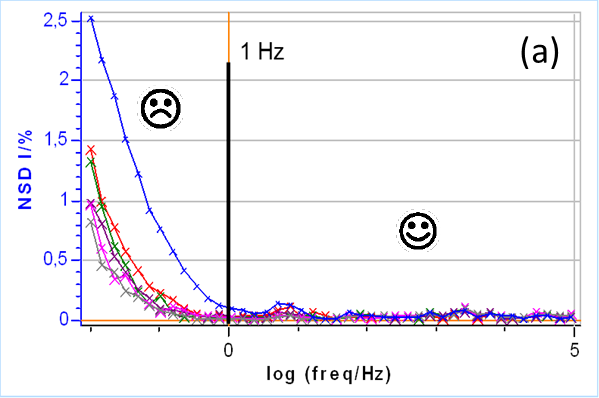

Figure 7: (a) NSD of the current response as a function of the frequency and (b) the corresponding impedance measurements. The 1 Hz boundary is also shown on both graphs, which could be used as a threshold value to separate quasi-stationary and non-stationary impedance data.
We have seen in this part that the NSD indicator could be used to indicate the non-stationarity of the system, which can lead to strong deformation of the impedance data and incorrect interpretation.
In the next part of the note we will explain the “4D impedance” method used to correct the effect of time-variance on impedance data which lead to data that can be considered as valid or quasi-stationary and correctly interpreted. The Z Inst analysis tool from EC-Lab® is used to perform and show the results.
“4D impedance” using Z Inst analysis tool from EC-Lab®
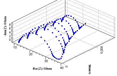
This method was first introduced by Stoynov in his seminal paper [16]. Firstly, the acquired impedance data need to be represented as a function of time as is shown in Fig. 8a, for the results from Fig. 4a.
Secondly, all data points obtained at the same frequency but at different times are interpolated to produce what we could name a temporal impedance envelope. For each frequency, $\text{Re}(Z)$ and $-\text{Im}(Z)$ are expressed as a function of time.
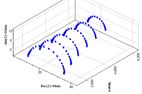
Thirdly, the instantaneous impedance is calculated considering it is a cross-section of the temporal impedance envelope. The time interval $\Delta t$ between each cross-section is:
$$\Delta t=(t_2-t_1)/n \tag{2}$$
With $t_2$ the time of the first data point of the last impedance graph, $t_1$ the time of the last data point of the first impedance graph, $n$ the number of chosen cross-sections, in the case of Fig. 8b, six.
These data, corrected for time-variance, can now be considered valid or quasi-stationary and could be interpreted using equivalent circuit modelling for example.
a)
b)
Figure 8: (a) Impedance data from Fig. 3a plotted as a function of time, b) Calculated instantaneous impedance diagrams.
Conclusion
In this paper, we showed the effect of system time-variance on impedance measurements and presented tools available in EC-Lab® to both detect and correct these effects. Experimental data obtained on a mild steel sample in sulfuric acid showed how the change of polarization resistance could strongly affect the data especially at lower frequencies. We presented several methods to check that impedance measurements are performed on a stationary system :
- performing successive measurements. If the graphs are the same then the system is stationary.
- using the NSD indicator. In the case of a non-stationary system, this indicator can be used to determine a lower frequency limit above which the data can be considered as valid. It is also recommended in corrosion to use galvano-controlled EIS so that the change of corrosion potential is accounted for.
Finally, the “4D impedance” method and its implementation in EC-Lab®, the Z Inst analysis tool, were described in detail, and demonstrated on corrosion data. This seems to be the only method to easily remove the effect of time-variance. The table below summarizes the tools available to check and correct non-stationarity in EIS measurements.
Table I: Tricks and tips to deal with non-stationarity in EIS measurements.
| Tool | Use |
|---|---|
| Perform successive EIS measurement | If the graphs are identical, the system is stationary, if not let it settle |
| Use the drift correction tool | Correct the non-stationarity of the system |
| Perform GEIS-AA measurements | Reduce the effect of time-variance |
| Measure NSD | Estimate the degree of non-stationarity |
| Perform Z Inst analysis | Remove the effect of time variance |
References
[1] M. Urquidi-Macdonald, D. Mac-donald, Electrochim. Acta 35 (1990) 1559
[2] K. Darowicki, J. Electroanal. Chem. 486 (2000) 101
[3] C. A. Schiller, F. Richter, E. Gülzow, N. Wagner, Phys. Chem. Chem. Phys., 3 (2001) 374
[4] C. Wagner and W. Traud, Z. für Elektrochemie und angewandte physikalische Physik 44 (1938) 391
[5] M. Stern and A. L. Geary, J. Electroch. Soc. 104 (1957) 56
[6] I. Epelboin, M. Keddam, H. Takenouti J. App. Electrochem. 2 (1972) 71
[7] F. Mansfeld in Advances in corrosion science and technology M. G. Fontana et al. Eds., Plenum Press, New York, U.S.A., 1976, p. 163
[8] C. Gabrielli, M. Keddam, H. Takenouti in Treatise on materials science and technology; Corrosion: aqueous processes and passive films, J. C. Scully, Ed., Academic Press Inc., London, U.-K., 1983, p. 395
[9] Application Note 69 Part II
[10] J.-P. Diard, P. Landaud, B. Le Gorrec, C. Montella, J. Electroanal. Chem. 255 (1988) 1
[11] N. Murer, J.-P. Diard, B. Petrescu, J. Electrochem. Sci. Eng. 10 (2020) 127
[12] BioLogic Application Note 55
[13] BioLogic Application Note 49
[14] BioLogic White Paper 2: systems and EIS quality indicators
[15] BioLogic Application Note 17
[16] Z. B. Stoynov, B. S. Savova-Stoynov, J. Electroanal. Chem, 183 (1985) 133
Revised in 11/2020
Data are available in:
C:\Users\…\Documents\EC-Lab\Data\Samples\EIS\AN69_I_DATA
Scientific articles are regularly added to BioLogic’s Learning Center:
To access all BioLogic’s application notes, technical notes and white papers click on Documentation:


