

How to check and correct non-stationary EIS measurements using EC-Lab® (Part 2) Battery – Application Note 69-2
Latest updated: June 4, 2024Abstract
This application note presents the various tools available in EC-Lab® that can be used to check and correct the non-stationarity of your EIS measurements. Using the proprietary Non-Stationary Distortion indicator and the instantaneous impedance analysis tool Z Inst, users can ensure that EIS measurements are correctly interpreted and fitted. This application note shows the use of such tools on data obtained on an LFP battery under discharge.
How to check and correct
non-stationary EIS measurements using EC-Lab®?
Part II: an example on a battery cell.
Introduction
For valid Electrochemical Impedance Spectroscopy (EIS) measurements, the system under investigation should be linear, stable, causal and stationary [1,2]. In this note, the term “stationarity” comprises steady-state and time-invariance.
Steady-state is the state of a system after its transient state. For example, an R/C circuit submitted to a potential or current step is in a transient state and sees its response change until a certain amount of time has passed.
Time-variance refers to a system whose parameters defining its transfer function change with time. The chemical composition of a battery cell’s electrodes changes during charging or discharging, which affects its impedance.
The two properties may be difficult to separate.
EIS measurements during continuous charge or discharge, or in operando, are used to inspect a battery under operation [3-8]. The problem with such cases is understanding which impedance data can be considered valid, or moreover, for which frequencies, data should be considered erroneous because of the non-stationarity of the system.
In this second application note, we will present various tools implemented in EC-Lab® to help check and correct the non-stationarity of the measurements. These tools will be applied to data obtained on a discharging battery.
Experimental conditions
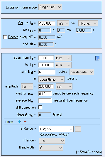
A 26650 LFP battery cell from A123 was used. A discharge of -100 mA during 130 s was performed followed by a galvano-controlled EIS (GEIS) measurement with a DC current of -100 mA and an AC current modulation of -200 mA at frequencies ranging from 1 kHz to 10 mHz with 6 points per frequency decade. Using a Loop technique, the experiment, composed of a discharge followed by a GEIS, was performed nine times (Fig. 1)

Figure 1: Parameters of the GEIS experiment performed on the 26650 LFP A123 battery cell.
Results
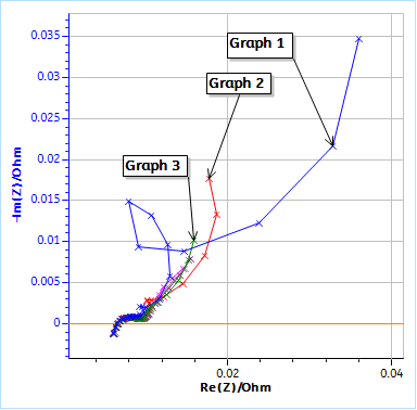
Figure 2 shows the successive impedance diagrams obtained on the batteries under discharge. Before each impedance measurement, the battery is discharged during 130 s at -100 mA. The impedance measurement is performed with galvanic control, hence there is no discontinuity between the discharge and the impedance measurement.
a)
b)
Figure 2: Nyquist plots of the impedance data obtained on a LFP 26650 cell using the conditions in Fig. 3. a) Full graph for cycle 1, 2, 3, 4, 5 and 9, b) Close-up at high frequencies. Each GEIS measurement was preceded by a discharge at -100 mA during 130 s.
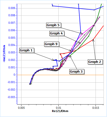
Figure 2a shows the totality of the chosen Nyquist diagrams (Cycle 1, 2, 3, 4, 5 and 9) and Figure 2b is a close-up on the high frequency part. The first three diagrams are quite different and then the data seem to stabilize.
Figure 3 shows the DC cell voltage evolution during the discharge and the impedance measurement for cycles 1 to 5, and 9.

Figure 3: DC Potential evolution obtained on a LFP 26650 battery from A123 during EIS measurements preceded by a discharge at -100 mA during 130 s.
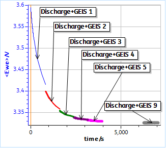
We can see that the potential mostly decreases during the first three cycles and then starts to stabilize.
The comparison of Figs. 2a and 3 shows that the unusual impedance values at low frequencies are due to the non-stationarity of the system, which is directly related to the DC current applied to the battery. It is quite difficult to interpret these data, and the peculiar shape of the impedance data at lower frequencies is not related to a specific electrochemical phenomenon but to the change of the systems parameters and a transient behavior.
Contrarily to a corroding system, which, for example, sees its polarization resistance changes with time [9,10], the chemical changes occurring in a battery while it is discharging are numerous and not easy to simulate and predict.
Which data can be reliably interpreted and considered as valid? How can it be made sure that the data interpretation is not erroneous? In the next part of this paper, we will present the tools available in EC-Lab® that may help address such problems.
How to check and correct time-variance using EC-Lab®
Non-Stationary Distortion (NSD) indicator
In this paper, as explained in the introduction, what we mean by non-stationarity is two-fold:
- The fact that the system is in a transient regime, that it has not yet reached its steady-state. Its transfer function stays the same throughout the experiment but its steady-state response is not reached instantaneously, it is lagging.
- The fact that the system sees its transfer function or the values of the parameters constituting its transfer function change over time. This is the time-variance we spoke of throughout the paper.
Both phenomena have a specific effect on the response signal, which can be seen on the impedance diagram, but also on its Fourier Transform (FT), which gives a frequency representation of the signal. The FT of the time response signal of a stationary (and linear) system will show a line at the same frequency as the input signal. The response of a non-stationary system, whether it is in a transient state or time-variant will show lines not only at the same frequency as the input signal but also at adjacent frequencies.
The amplitude of the adjacent lines around the signal response at the fundamental frequency depends on the extent of the non-stationarity of the system.
We can introduce an indicator that can be used to quantify the non-stationarity of the signal, whether it is due to a transient state or to a time-variance. We call this indicator NSD. It is calculated as follows:
$$\text{NSD}(f)=\frac{1}{Y_f}\sqrt{Y_{f-\Delta f}^2+Y_{f+\Delta f}^2}\tag{1}$$
where $Y_f$ is the amplitude at the stimulation or fundamental frequency $f$, $Y_{f-\Delta f}^2$ and $Y_{f+\Delta f}^2$ are the amplitudes at the frequencies adjacent to the fundamental $f-\Delta f$ and $f+\Delta f$, and $\Delta$ f is the spectral frequency resolution.
All this is illustrated and explained in more details in the corresponding BioLogic white paper [11].
Please also note that the “drift correction” tool, shown in Fig. 6 can be used to account for and correct the non-stationarity of the system [12].
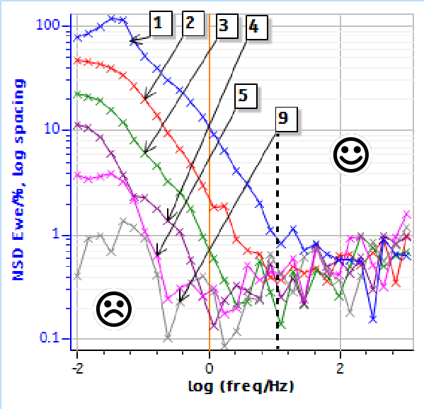
Figure 4 shows the NSD of the potential response for impedance data measured on a discharging battery shown in Fig. 2. It is clear that the conditions are highly non-stationary with a NSD reaching a maximum of 120% at around 100 mHz for the first measurement (Fig. 2a) where the DC potential changes the most (Fig. 3).
The maximum NSD is reduced drastically for the second measurement reaching 50% at 10 mHz (Fig. 4). The maximum NSD does not go over 4% at all frequencies from the fifth measurement (Fig. 4).

Figure 4: NSD of the potential response from impedance measurements shown in Fig. 2a and 2b. The dashed line indicates the 10 Hz limit between non-stationary and quasi-stationary data.
At this point, the potential does not change along the measurement (Fig. 3), as we have reached the nominal potential of the battery.
At the ninth measurement, the NSD is very close to 0% for all frequencies (Fig. 4). In the same way as for the impedance measurement on a corroding system [13], we can determine a lower frequency limit below which we consider that the measurements are not valid and cannot be interpreted without accounting for non-stationarity.
In the case of the measurement on the battery cell, this lower limit would be 10 Hz. It is indicated as a straight and dashed line in Fig. 4.
We have seen in this part of the application note that the NSD indicator could be used to indicate the non-stationarity of the system, which can lead to strong deformation of the impedance data and incorrect interpretation.
In the next part of the note we will explain the “4D impedance” method to correct the effect of time-variance on impedance data which lead to data that can be considered as valid or quasi-stationary and correctly interpreted. The Z Inst analysis tool from EC-Lab® is used to perform and show these results.
“4D impedance” using Z Inst analysis tool from EC-Lab®
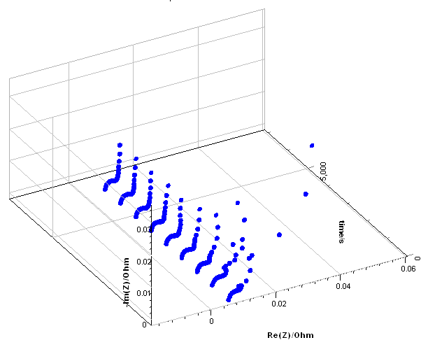
This method was first introduced by Stoynov in his seminal paper [14]. Firstly, the acquired impedance data need to be represented as a function of time as is shown in Fig. 5a for the results from Fig. 2.
Secondly, all data points obtained at the same frequency but at different times are interpolated to produce what we could name a temporal impedance envelope. For each frequency, $\text{Re}(Z)$ and $-\text{Im}(Z)$ are expressed as a function of time.
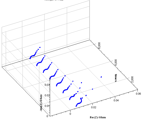
Thirdly, the instantaneous impedance is calculated considering it is a cross-section of the temporal impedance envelope. The time interval $\Delta t$ between each cross-section is:
$$\Delta t=(t_2-t_1)/n \tag{2}$$
With $t_2$ the time of the first data point of the last impedance graph, $t_1$ the time of the last data point of the first impedance graph, $n$ the number of chosen cross-sections, in the case of Fig. 5b, eight. Figure 5b shows $\text{Re}(Z)$ vs. $t$ for the experimental data (dots) and the corrected data (lines+crosses).
a)
b)
c)
Figure 5: a) Impedance data from Fig. 2a plotted as a function of time, b) Calculated instantaneous impedance diagrams c) $\text{Re}(Z)$ vs. $t$ for experimental data (dots) and corrected data (lines+crosses).
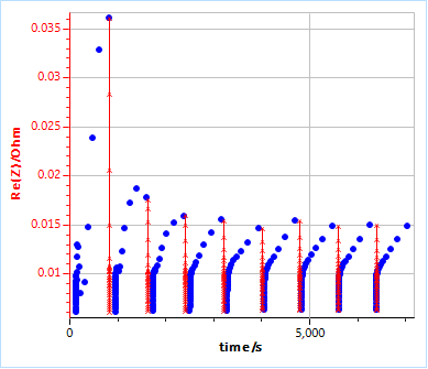
These data, corrected for time-variance, can now be considered valid or quasi-stationary and could be interpreted using equivalent circuit modelling.
Conclusion
In this paper, we showed the effect of system time-variance on impedance measurements and presented the tools available in EC-Lab® to both detect and correct these effects.
We also showed some data obtained on a discharging battery. Impedance data can be considered stationary when the nominal voltage of the battery is reached.
Several methods available to check that impedance measurements are performed on a stationary system or not were presented:
- performing successive measurements. If the graphs are the same then the system is stationary
- using the NSD indicator. This indicator is also used to determine a lower frequency limit below which the data cannot be considered as valid. It is also recommended in corrosion to use galvano-controlled EIS so that the change of corrosion potential is accounted for.
Finally, the “4D impedance” method and its implementation in EC-Lab®, the Z Inst analysis tool, were described in detail, and used on the battery data. It seems to be the only method to easily remove the effect of time-variance.
The table below summarizes the tools available to check and correct non-stationarity in EIS measurements.
The data shown in this application note can be found in:
C:\Users\…\Documents\EC-Lab\Data\Samples\EIS\AN69_II_DATA
Table I: Tricks and tips to deal with non-stationarity in EIS measurements.
| Tool | Use |
| Perform successive EIS measurement | If the graphs are identical, the system is stationary, if not, let it settle |
| Use the drift correction tool | Correct the non-stationarity of the system |
| Perform GEIS-AA measurements | Reduce the effect of time-variance |
| Measure NSD | Estimate the degree of non-stationarity |
| Perform Z Inst analysis | Remove the effect of time variance |
References
[1] M. Urquidi-Macdonald, D. Mac-donald, Electrochim. Acta 35 (1990) 1559
[2] K. Darowicki, J. Electroanal. Chem. 486 (2000) 101
[3] Z. B. Stoynov, B. S. Savova-Stoynov, J. Electroanal. Chem, 183 (1985) 133
[4] F. Berthier, J.-P. Diard, A. Jussiaume, J.-J. Rameau, Corrosion Science, 30 (1990) 239
[5] M. Keddam, Z. B. Stoynov, H. Takenouti, J. App. Electrochem. 7 (1977) 539
[6] M. Itagaki, K. Honda, Y. Hoshi and I. Shitanda, J. Electroanal. Chem. 737 (2015) 78
[7] M. Itagaki, N. Kobari, S. Yotsuda, K. Watanabe, S. Kinoshita, M. Ue, J. Power Sources 135 (2004) 255
[8] J.-P. Diard, B. Le Gorrec, C. Montella, J. Power Sources, 70 (1998) 78
[9] N. Murer, J.-P. Diard, B. Petrescu, J. Electrochem. Sci. Eng. 10 (2020) 127
[10] BioLogic Application Note 55
[11] BioLogic White Paper 2: systems and EIS quality indicators
[12] BioLogic Application Note 17
[13] BioLogic Application Note 69 Part I
[14] Z. B. Stoynov, B. S. Savova-Stoynov, J. Electroanal. Chem, 183 (1985) 133
Revised in 11/2020
Scientific articles are regularly added to BioLogic’s Learning Center:


