

How to interpret lower frequencies impedance in batteries (EIS low frequency diffusion) Battery – Application Note 61
Latest updated: December 11, 2024Abstract
The lower frequencies part of the impedance is of interest as it can be used to derive critical characteristics such as the diffusion constant of the intercatalated species in a given material. This note explains in which conditions this parameter can calculated from impedance data.
Introduction
Impedance measurements can be used to monitor and control the degradation of the battery performance during cycling. Measurements are usually performed at higher frequencies to determine the internal resistance of an element [1-4].
However, in the case of batteries involving intercalation of species, at lower frequencies, impedance measurements can also prove to be useful as in certain conditions it is possible to extract the diffusion coefficient of the intercalated species. This quantity is also of great importance to the process of quality optimization and monitoring of battery materials [3-6].
This application note gives examples on how impedance data at lower frequencies can be fitted and the method to extract useful experimental data by selecting the most appropriate element for the Equivalent Circuit (EC).
It also implicitly shows that impedance measurements are fully beneficial only when performed over a frequency range and not at a single frequency.
It must be noted that the following study was performed using the two poles of commercial batteries. To be able to interpret data, it is assumed that the impedance of one electrode is negligible compared to the other and that the impedance graphs shown are related to one pole or one electrode of the battery.
Impedance Results
Figure 1 below shows the impedance graphs obtained on three different new commercial Li-ion batteries with 100% State Of Charge (SOC):
- UltraFire BRC18650 3.7 V, 3000 mAh
- Panasonic NCR18650B 3.6 V, 3200 mAh
- Samsung ICR18650 3.7 V, 3000 mAh
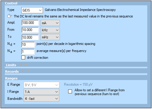
The impedance graphs shown in Fig. 1 were obtained using a Bio-Logic BCS-815 and BT-Lab® 1.30. The same experiment could be performed using an EIS capable Bio-Logic potentiostat/galvanostat. The conditions are shown in Fig. 2.

Figure 1: Impedance graphs obtained on the three different batteries and used as fitting examples in this note.
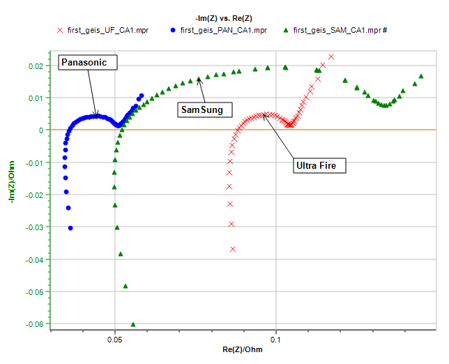

Figure 2: Conditions used in the ModuloBat technique to obtain the impedance graphs shown in Fig. 1. DC current level is 0 A.
How To Fit Data At Low Frequencies
The Issue
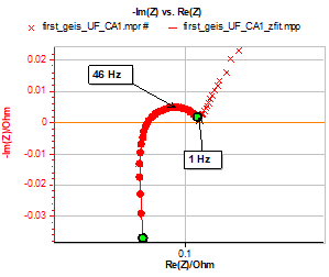
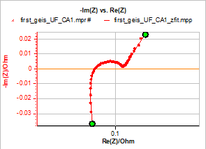
The impedance data shown in Fig. 3 for the Ultra Fire battery lead us to say that data from 10 kHz to around 1 Hz (just before the low frequencies increase) can be fitted with the following equivalent circuit:
R1+R2/L2+R3/Q3+R4/Q4. The result of this fit, performed with ZFit is shown in Fig. 3.
Randomize+Simplex was used as a minimization algorithm over 15000 iterations for the Randomize process and 30000 iterations for Simplex. The minimization criterion, namely χ², criterion was not weighted.
A number of elements could be chosen to fit data below 1 Hz. ZFit offers many elements: Q, W, M, Mg and Ma.
The expression of the impedance and the shape of the impedance curve for each element are recalled in the following part and in the Appendix, respectively.
The relevance of each element is also discussed based on three questions:
- Can it be used to fit the data?
- Which element leads to the best fit?
- Which element can be physically interpreted and give access to a physical quantity?

Figure 3: Impedance graph and fit from 10 kHz to 1 Hz. Equivalent circuit: R1+R2/L2+R3/Q3+R4/Q4. Parameters used for the fit: R1 = 0.084 Ω, R2 = 0.80 Ω, L2 = 0.61×10⁻⁶ H, R3 = 5.18×10⁻³ Ω, Q3 = 0.087 F s(a3-1), a3 = 0.88, R4 = 0.015 Ω, Q4 = 1.17 F s(a4 – 1), a4 = 0.71.
Q
The impedance of the element Q also known as Constant Phase Element (CPE) is expressed as:
$$Z_\text{CPE}(f)= \frac{1}{Q(j2\pi f)^\alpha}\tag{1}$$
where Q is the CPE with the unit F sα-1, is the frequency in Hz, α ∈ [0, 1] and j is the imaginary number j² = -1.
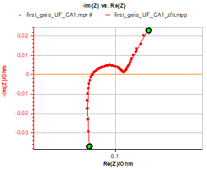
An example of an impedance graph fitted with the equivalent circuit given in III-1 with the addition of the Q element is given in Fig. 4 for the Ultra Fire battery.

Figure 4: Impedance graph and fit from 10 kHz to 1 Hz. Equivalent circuit: R1+R2/L2+R3/Q3+R4/Q4+Q5. Parameters used for the fit: R1 = 0.084 Ω, R2 = 0.76 Ω, L2 = 0.61×10⁻⁶ H, R3 = 7.1×10⁻³ Ω, Q3 = 0.15 F s(a3-1), a3 = 0.8, R4 = 0.013 Ω, Q4 = 1.05 F s(a4 – 1), a4 = 0.78, Q5 = 266 F s(a5-1), a5 = 0.69; χ² = 1.8×10⁻⁶ Ω².
The admitted and most common physical interpretation of the CPE element is the microstructural heterogeneity of the electrode which causes a distribution of the current densities, and capacitances along the electrode surface [7]. A CPE does not give any information about transport phenomena, which is critical in the field of batteries.
The parameter χ², used as a minimization criterion, reflects the goodness of the fit. As a reminder, χ² is calculated in ZFit with the following relationship:
$$\chi^2= \frac{1}{N}\sum^{N}_{i=1}|Z_i(f_i)-Z(f_i)|^2\tag{2}$$
with Zi the measured impedance and Z(fi) the value of the impedance calculated at a frequency fi for a defined set of parameter values and N the number of points. The fitting algorithm tries to find the values of each parameter for which the parameter χ² is minimized. The lower the χ², the better the fit. The comparison of this parameter between each battery technology will be given in Part III-4.
W
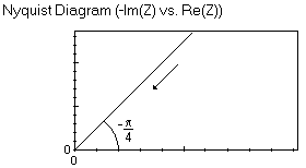
In the particular case where, in Eq. (1), α = 0.5, the impedance is analogous to that of the Warburg element W:
$$Z_\text{W} (f)=\frac{\sqrt{2}\sigma}{\sqrt{(j2\pi f)}}\tag{3}$$
with σ the Warburg parameter in Ω s-1/2.
The Warburg element is representative of a semi-infinite linear diffusion and it may seem erroneous to consider intercalation as a semi-infinite process as the intercalation material is finite in space.
Nonetheless, within a certain frequency range (i.e. not too low) the Warburg impedance could be considered as valid and used to extract the diffusion coefficient as:
$$\sigma = \frac{RT}{n^2F^2AX^*\sqrt{2D_\text{X}}}\tag{4}$$
with A the area of the electrode, X* and DX the bulk concentration and the diffusion coefficient of the species X, respectively, in our case Li+.
In order to use Eq. (4), we would need to know the bulk concentration of Li+ in the electrolyte.
It would also be assumed that the impedance of the positive electrode is negligible compared to the negative electrode in which the Li+ are inserted and that the diffusion mechanism highlighted in the impedance graph only reflects the mechanism occurring on the negative electrode.
Figure 4 shows that the a5 parameter is around 0.7, which means that the graph cannot be fitted with a Warburg element at low frequencies. A value of 0.5 means that the impedance curve is a straight line forming a -π/4 angle with the real axis, as is recalled in the Appendix.
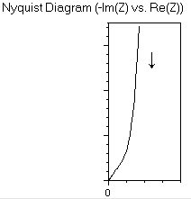
M
This element is used to describe linear restricted diffusion, i.e. diffusion of an element in an electrode with a definite thickness δ.
The impedance of this element writes:
$$Z_\text{M}(f)=R_\text{d}\frac{\text{coth}\sqrt{\tau_\text{d}j2\pi f}}{\sqrt{\tau_\text{d}j2\pi f}}\tag{5}$$
With τd the diffusion time constant in s, and Rd the resistance associated with the restricted linear diffusion mechanism.
As it can be seen in the Appendix the impedance curve is at high frequencies a straight line making an angle of -π/4 with the real axis as seen with the Warburg element and at low frequencies a vertical line. Hence, similarly to the W element, the M element cannot be used to fit the data.
Nonetheless, M is more interesting than the W element as the value of the diffusion time constant τd is more directly related to the diffusion coefficient D by:
$$\tau_\text{d}=\frac{\delta^2}{D_\text X}\tag{6}$$
where δ is the thickness of the electrode in which the species X with a diffusion coefficient DX is inserted.
If it is assumed that the impedance of one electrode is negligible, we can have a direct access to the diffusion coefficient of the species in the other electrode. The M element is more convenient as the thickness of the electrode is more accessible than the bulk concentration of the species.
Ma
This element is used to describe linear modified restricted diffusion. The expression of the impedance is based on the impedance of the element M only with an additional factor α called a dispersion parameter [8].
$${Z_\text{Ma}}(f)=R_\text{d}\frac{\text{coth}(\tau_\text{d}j2\pi f)^{\alpha/2}}{(\tau_\text{d}j2\pi f)^{\alpha/2}}\tag{7}$$
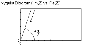
The impedance of the element Ma has two components: at higher frequencies a straight line that forms an angle of -απ/4 with the real axis and at lower frequencies a straight line forming an angle of -απ/2 with the real axis. The results of the fitting obtained with this element is shown in Fig. 5.

Figure 5: Impedance graph and fit from 10 kHz to 1 Hz. Equivalent circuit: R1+R2/L2+R3/Q3+R4/Q4+Ma5. Parameters used for the fit: R1 = 0.084 Ω, R2 = 0.75 Ω, L2 = 0.61×10⁻⁶ H, R3 = 0.012 Ω, Q3 = 1.07 F s(a3-1), a3 = 0.78, R4 = 7.54×10⁻³ Ω, Q4 = 0.18 F s(a4 – 1), a4 = 0.78, Rd5 = 2.82×10⁻⁹ Ω, td5 = 1.2×10⁻⁹ s, a5 = 0.69; χ² = 1.8×10⁻⁶ Ω².
Similarly, the diffusion coefficient can be readily obtained using Eq. (6).
Mg
The anomalous linear diffusion impedance element can also be used in the case where the impedance graph does not exhibit a straight line with a -π/4 angle with the real axis at low frequencies as it is the case for each graph shown in this publication. The shape of the impedance graph is shown in the Appendix.
The impedance of the Mg element is a more general example of the restricted diffusion impedance and writes [9]:
$${Z_\text{Mg}}(f)=R_\text{d}\frac{\text{coth}(\tau_\text{d}j2\pi f)^{\gamma/2}}{(\tau_\text{d}j2\pi f)^{1-\gamma/2}}\tag{8}$$
with γ a parameter lower or equal to 1.
One can note that if γ = 1, Eqs. (8) and (5) are the same.
The results of the fitting obtained with this element is shown in Fig. 6.

Figure 6: Impedance graph and fit from 10 kHz to 1 Hz. Equivalent circuit: R1+R2/L2+R3/Q3+R4/Q4+Mg5. Parameters used for the fit: R1 = 0.084 Ω, R2 = 0.77 Ω, L2 = 0.61×10⁻⁶ H, R3 = 7.1×10⁻³ Ω, Q3 = 0.15 F s(a3-1), a3 = 0.80, R4 = 0.013 Ω, Q4 = 1.05 F s(a4 – 1), a4 = 0.78, Rd5 = 0.55 Ω, td5 = 1430 s, g5 = 0.63; χ² = 1.8×10⁻⁶ Ω².
Similarly, a relationship exists between the time constant and the diffusion coefficient of the inserted species, but it is weighted by the parameter γ as shown below:
$$\tau_\text{d}=\left(\frac{\delta^2}{D_X}\right)^{1/\gamma}\tag{9}$$
As for the M and Ma elements one only needs to know the thickness of the electrode to determine the diffusion coefficient.
Discussion
a. Element that can be used for fitting
As noted above, the W and M cannot be used for fitting lower frequencies impedance of the batteries used here. Remaining candidates are: Q, Ma and Mg
b. Quality of the fit: χ2 comparison
Table I shows the values of the Χ² parameter for each battery for each element chosen to model impedance at low frequencies (<1 Hz): Q, Ma or Mg. It must be noted that the unit of χ² is Ω² and consequently depends on the actual values of the impedance measured. For this reason, the χ² cannot be quantitatively compared bet-ween each battery type.
Table I: χ² values for each battery and each element used to model impedance at low frequencies.
| χ²/(10-6 Ω²) | Ultra Fire | Samsung | Panasonic |
|---|---|---|---|
| Q | 1.82 | 23.9 | 0.86 |
| Ma | 1.82 | 23.7 | 0.86 |
| Mg | 1.80 | 23.7 | 0.78 |
If we base our comparison only on the quality of the fit, it seems that a slightly better fit is performed for the UltraFire and Panasonic batteries using the Mg element.
For Samsung batteries, all three elements lead to the same fit quality.
In summary, the examination of χ² cannot lead to a clear discrimination and the remaining candidates are still Q, Ma and Mg
c. Physical relevance
Q could be a good candidate, but it lacks physical meaning when attempting to interpret data.
Ma and Mg are beneficial because they allow an extraction of the diffusion constant, just by knowing the electrode thickness and using Eqs. (6) and (9), respectively (and assuming that only the impedance of the considered electrode is measured, without the contribution from the positive electrode).
DX is obtained from Eq. (9):
$$D_\text{X}=\frac{\delta^2}{\tau_\text{d}^\gamma}\tag{10}$$
Tab. II shows the diffusion constants obtained for the three batteries assuming a thickness of the negative electrode of ca. 70 µm. Table IIa and IIb show the results for Ma and Mg, respectively.
Typical values for diffusion constants in solids are at the order of magnitude of 10-10 cm2 s-1 [6], hence it seems that the values given by fitting Ma element are totally erroneous. This could also be inferred from the values of the Rd and τd in the fitting results shown in Fig. 6.
The only remaining element for fitting is the element Mg.
Table II: Diffusion constants values deduced from impedance fitting and a) Eq. (6) for Ma and b) Eq. (10) for Mg.
a)
| For element Ma | Ultra Fire | Samsung | Panasonic |
|---|---|---|---|
| τd/s | 1.19×10⁻⁹ | 1.704 | 11.9×10⁻⁶ |
| α | 0.69 | 0.59 | 0.60 |
| DX/(cm2 s-1) | 41176 | 2.88×10⁻⁵ | 4.12 |
b)
| For Element Mg | Ultra Fire | Samsung | Panasonic |
|---|---|---|---|
| τd/s | 1431 | 478 | 179 |
| γ | 0.628 | 0.829 | 0.785 |
| DX/(cm2 s-g ×10-9) | 511 | 294 | 835 |
| DXapp/(cm2 s-1 ×10⁻⁹) | 34.2 | 103 | 273 |
As noted in [10], the dimension of DX obtained by fitting the Mg element is not the usual dimension (cm2s-1).
One can get around this by calculating an apparent chemical diffusion coefficient DXapp by assuming γ = 1 in Eq. (10).
The obtained values (Tab. IIb) are lower than DX values. They are also one or two order of magnitudes higher than the values obtained in [6] for LiMnO2 batteries and in [11-12] for LiFePO4 batteries.
Values of Li+ diffusion in MesoCarbon-MicroBead (MCMB) single particle electrode have been reported to be within a range of 10-6-10-11 [13].
Discrepancies could be explained by various factors such as the contribution of the other electrode on the measured impedance, the influence of the state of charge of the battery and the lack of information about the precise battery technology and geometry.
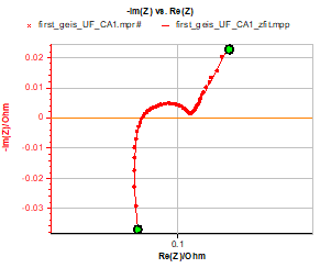
Finally, it should be noted that the method exposed here is much more relevant and consistent if the impedance graph contains data points at frequencies lower than 1 Hz. Not so much in order to obtain the typical shape of the impedance graph (for example, the “elbow” in the case of the M element) but because at higher frequencies of the diffusion process, the parameters Rd and τd can be indistinguishable and fitting can lead to erroneous values.
Figure 7 shows an example of such a typical graph.

Figure 7: Impedance graph and fit from 200 kHz to 10 mHz. Equivalent circuit: R1+L1+R2/Q1+Ma3. Parameters used for the fit: R1 = 0.025 Ω, L1 = 36.3×10⁻⁹ H, R2 = 0.062 Ω, Q1 = 7.9×10⁻³ F s(a1 – 1), a1 = 0.88, R3 = 0.088 Ω, t3 = 16.2 s, a3 = 0.735, χ² = 0.9×10⁻⁴ Ω².
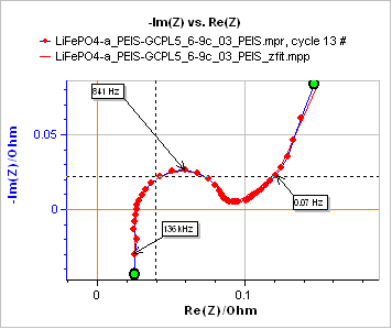
Using Eq. (6), the value of the time constant shown in Fig. 7 and the thickness of electrode, one can deduce the diffusion coefficient of the considered species.
Conclusion
Many elements are available in EC-Lab®’s ZFit to fit the low frequency component of impedance spectra obtained on batteries. Based on graphs obtained on three commercial batteries, a method was proposed to help select the best element and show how the chemical diffusion coefficient can be calculated using the results of the fit and making a few experimental assumptions.
The anomalous diffusion element was shown as the best candidate to fit low frequency data. The calculated diffusion coefficient was somewhat larger than most common values but still within a sensible range.
Data files can be found in :
C:\Users\xxx\Documents\EC-Lab\Data\Samples\Battery\ AN61_first_geis_X
Appendix
More information is given in the Handbook of Electrochemical Impedance Spectroscopy [14].
Q
W
M

Ma

Mg
References
1) P. Arora, R. E. White, J. Electrochem. Soc., 145, 10 (1998) 3647.
2) J. Vetter, P. Novák, M.R. Wagner, C. Veit, K.-C. Möller, J.O. Besenhard, M. Winter, M. Wohlfahrt-Mehrens, C. Vogler, A. Hammouche, J. Power Sources, 147 (2005) 269.
3) U. Tröltzsch, O. Kanoun, H.-R. Tränkler, Electrochim. Acta 51 (2006) 1664.
4) M. Mirzaeian, P. J. Hall, J. Power Sources 195 (2010) 6817.
5) M. Quintin, O. Devos, M.H. Delville, G. Campet, Electrochim. Acta 51 (2006) 6426.
6) H. Manjunatha, K.C. Mahesh, G.S. Suresh, T.V. Venkatesha Electrochim. Acta 56 (2011) 1439.
7) G. J. Brug, A. L. G. Van Den Eeden, M. Sluyters-Rehbach, J.H. Sluyters, J. Electroanal Chem. 176 (1984) 275.
8) R. Cabanel, G. Barral, J.-P. Diard, B. Le Gorrec, C. Montella, J. Appl. Chem. 23 (1993) 93.
9) J. Bisquert, and A. Compte, J. Electroanal. Chem. 499 (2001) 112.
10) C. Montella, R. Michel, J. Electroanal. Chem. 628 (2009) 97.
11) M. D. Levi, R. Demadrille, A. Pron, M. A. Vorotyntsev, Y. Gofer, D. Aurbach, J. Electrochem. Soc. 152 (2005) E61.
12) P. P. Prosini, M. Lisi, D. Zane, M. Pasquali Solid State Ionics 148 (2002) 45.
13) M. Umeda, K. Dokko, Y. Fujita, M. Mohamedi, I. Uchida, J.R. Selman, Electrochim. Acta 47 (2001) 885.
14) Handbook of Electrochemical Impedance Spectroscopy « Diffusion Impedances »
Revised in 08/2019


