

Application of the Capacitance – Voltage curve to photovoltaic cell characterizations (EIS & CV curve) Photovoltaic – Application Note 35
Latest updated: July 31, 2023Abstract
This note describing how to collect and process photovoltaic impedance data in EC-Lab to generate a capacitance-voltage plot without any need for post-processing or fitting of the raw data. Using existing software features, a C-V plot is easily generated.
Introduction
Capacitance measurement is widely used to carry out semiconductor characterization such as those for photovoltaic (PV) cells. For example, this measurement is used to determine the doping concentration.
In EC-Lab® & EC-Lab® Express software, it is possible to directly plot the capacitance (directly means without any post-process). The capacitance can be obtained with all the Electrochemical Impedance Spectroscopy (EIS) techniques i.e. Potentio EIS (PEIS), Galvano EIS (GEIS), Staircase PEIS (SPEIS), Staircase GEIS (SGEIS), “Wait” technique that allows user to follow up the modulus of Z vs time (PEISW) techniques.
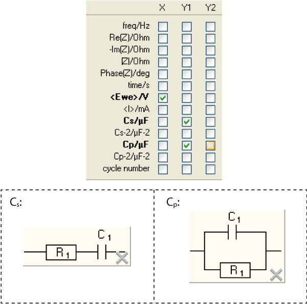
Depending on the model circuits considered, two types of capacitance, Cs or Cp, are calculated. The capacitance Cs corresponds to the capacitance of the R+C (in series) circuit and Cp corresponds to the capacitance of the R/C (in parallel) circuit (Fig. 1)

Figure 1: The two equivalent circuits offered for direct capacitance plotting.
This note demonstrates how to plot a Capacitance vs. Voltage (C–V) curve. Firstly, the different options offered to plot the capacitance are shown with a varia-capacitor as an experimental model system. A discussion is given about the selection of the circuit model and a comparison between the capacitance values fitted with ZFit and the capacitance directly available in the technique. Secondly, typical C-V characterizations of PV cell are described.
Experimental conditions
Investigations are carried out with a SP-200 equipped with the Ultra Low Current option or with SP-300 and EC-Lab® software. For both systems (i.e. varia-capacitor and photovoltaic cell), investigations were carried out with a standard two-electrode connection.
The characteristics of the varia-capacitor are described below:
- low voltage variable capacitance double diode (BB201 from NXP).
- The capacitance is in the range of 10 to 120 pF for a voltage range of 0.5 to 11 V.
The C–V characterization of the PV cell has been performed on a cell irradiated by a Xenon lamp of 150 W (light source of MOS-200 powered by ALX-150 power supply).
Varia-capacitor investigations
R/C or R+C Equivalent circuit?
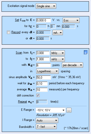
To choose the appropriate equivalent circuit among R/C or R+C, an EIS measurement on a wide frequency range i.e. 3 MHz to 1 mHz is performed. Settings are displayed in Fig. 2.
The EIS measurement leads to a semicircle (Fig. 3), so the R/C model (Cp variable) is considered for the C–V investigations. The fitted values of R and C are 70 Ohm and 145 pF (Fig. 4), respectively.

Figure 2: Settings for the EIS characterizations of the varia-capacitor.
C–V Investigations
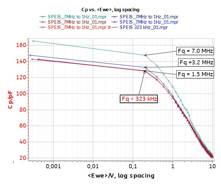
Two SPEIS techniques are performed. One in the frequency range from 7 MHz to 1 Hz (setting displayed in Fig. 5) and one at one frequency (with similar settings to those shown in Fig. 5 with fi equal to ff). Measurements were performed at a frequency of 323 kHz because above this frequency the responses of the varia-capacitor is dependent on the frequency (Fig. 6). The experiments are named SPEIS7MHz-1Hz and SPEIS323kHz, respectively. The voltage scan starts at 0 V and goes up to 10 V with steps of 200 mV.

Figure 3: Nyquist plot of varia-capacitor (Exp data fitted data).
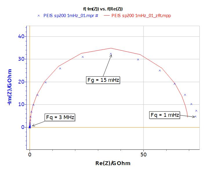

Figure 4: Values of the Zfit process.
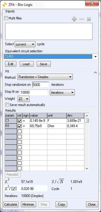

Figure 5: SPEIS settings for varia-capacitor characterizations.
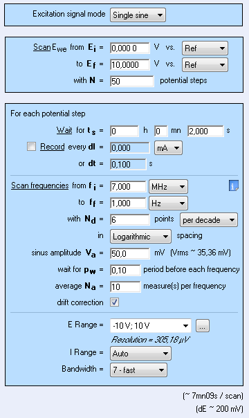
Figure 6: C–V characterization at different frequencies.
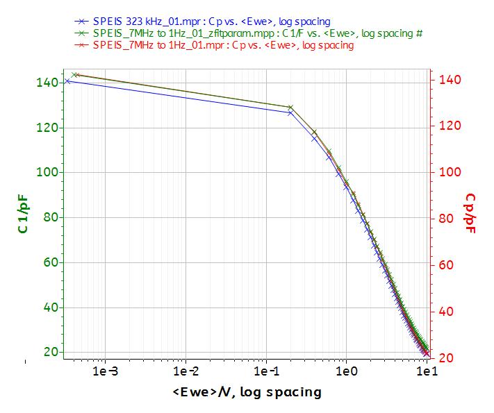
The SPEIS7MHz-1Hz allows users to fit the capacitance value, C1 with the Zfit tool at the different frequencies (window of frequency selection is displayed in Fig. 7). C1 is compared in Fig. 8 to the value of Cp that is already calculated during the experiments SPEIS7MHz-1Hz and SPEIS323kHz. C1 and Cp leads to similar values around 140 pF at low voltage and 20 pF at high voltage. So, the comparison shows that the C1 calculated with Zfit and Cp determined directly in the EIS technique are identical.
These values are in agreement with the specification described in the datasheet of the varia-capacitor.
Moreover, SPEIS7MHz-1Hz and SPEIS323kHz last 6,200 s and 150 s, respectively. So it is possible to save time by performing SPEIS at one frequency.

Figure 7: Frequency selection.
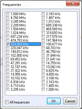
Figure 8: semi logarithmic C–V curves of varia capacitor. Cp vs E of SPEIS323kHz; Cp vs. E of SPEIS7MHz-1Hz and C1 (from Zfit) vs. E of SPEIS7MHz-1Hz.
C–V Curve of photovoltaic cell
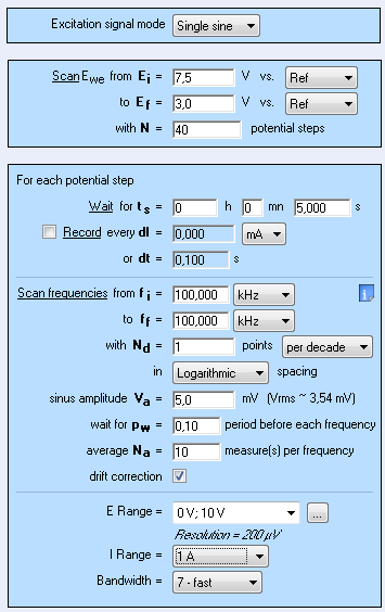
For the PV cell characterization, the voltage is scanned between 3 and 7.5 V and the frequency of the signal is 100 kHz (Fig, 9). According to the application note #24 [1], R/C model is considered. So Cp vs V curve is plotted (Fig. 10).
The C-V curve exhibits 3 regions:
- E < 4V: accumulation region
- 4V < E <6V: depletion region
- E > 6V: Inversion region

Figure 9: C–V curves settings of PV cell characterization.
The doping concentration N can be determined thanks to the following relationship:
$$N=\frac{2}{e\varepsilon\varepsilon_0A^2\left(\frac{d\left(\frac{1}{C^2}\right)}{dE}\right)} \tag{1}$$
Where e is the electron charge (1.60 x 10⁻¹⁹ C)
ε0 is the semiconductor permittivity (1.03 x 10⁻¹² F/cm for silicon)
A is the surface of the photovoltaic cell, 21 cm2
C is the capacitance (F) and E the voltage (V).
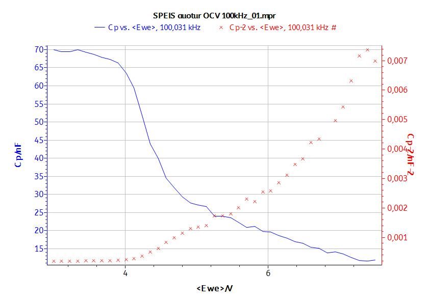
As C-2 variable is also available in the list of available variable (Fig. 1), it is also possible to plot C-2 vs. E. The slope of this curve leads to the doping concentration.
In this case, the slope (determined by linear fit) is 3.53 x 10¹⁵ F/V, so the doping concentration is 1.64 x 1014 cm-3. This value is in agreement with a value previously given [1].

Figure 10: C–V curves of photovoltaic cell. Cp vs. E and Cp-2 vs. E.
Conclusion
The note shows how to perform capacitance measurements without any fitting process. This offers several advantages:
- Quick measurement, only one frequency is needed to determine Cp or Cs. No need for the full EIS spectra.
- No post-treatment: no impedance fitting process is needed
- The graphic package of EC-Lab® allows one to plot different types of graph such as C vs. E in log spacing, C-2 vs. E, and even more…
It is possible to follow up the capacitance change that can be carried out with the PEISW technique. This technique is also of interest for sensor applications.
Data files can be found in :
C:\Users\xxx\Documents\EC-Lab\Data\Samples\Photovoltaic\X_C_V_Cha-ract
References
1) Application Note #24 “Photovoltaic Characterizations: Polarization and Mott-Schottky plot”
Revised in 08/2019


