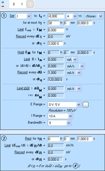
Supercapacitor characterization by galvanostatic polarization method (DC characterizations) Supercapacitor – Application Note 51

Introduction

Supercapacitors known as Electric Double Layer Capacitors (EDLCs) are used as energy storage devices for applications requiring power for short periods of time. Typically, an EDLC consists of two porous carbon-based electrodes electrically isolated by a porous separator. The separator and the electrodes are impregnated with an electrolyte, which allows the ionic current to flow between the electrodes while preventing electronic current from discharging the supercapacitor [1].

Compared to batteries, the supercapacitors are characterized by a quick charge and discharge regime, high power density and long cycle life. These devices are rated to support over one million cycles.

Many different methods are used to measure supercapacitor parameters: cyclic voltammetry, impedance spectroscopy, potentiostatic and galvanostatic methods. The first methods were explained in the application notes (#33) and (#34) [2-3].

The present note describes how to evaluate the characteristics of a supercapacitor (capacitance, capacity, energy, internal resistance and coulombic efficiency) using galvanostatic polarization method and the “Capacity & Energy per Cycle or Sequence” analysis tool available in EC-Lab^® software.

Experimental Conditions

The tested commercial supercapacitors are manufactured by two different companies: a PANASONIC gold supercapacitor (HW series) with a rated voltage of 2.3 V and a nominal capacitance of 22 F and an IOXUS supercapacitor with a nominal capacitance of 400 F and a rated voltage of 2.7 V, referred to as SC22 and SC400, respectively.

Each supercapacitor was cycled at ambient temperature (~ 19°C) between its rated voltage and 0 V using an SP-300 potentiostat/ galvanostat with a 10 A booster.

Supercapacitors were charged up to the rated voltage and then discharged to 0 V. Numerous charge/discharge rates were tested. The data were acquired and processed using EC-Lab^® software.

The galvanostatic polarization protocol used in this note is the GCPL technique.

Alternatively, the constant current (CstC) technique located in the supercapacitor section of EC-Lab^® can also be used for supercapacitor testing.

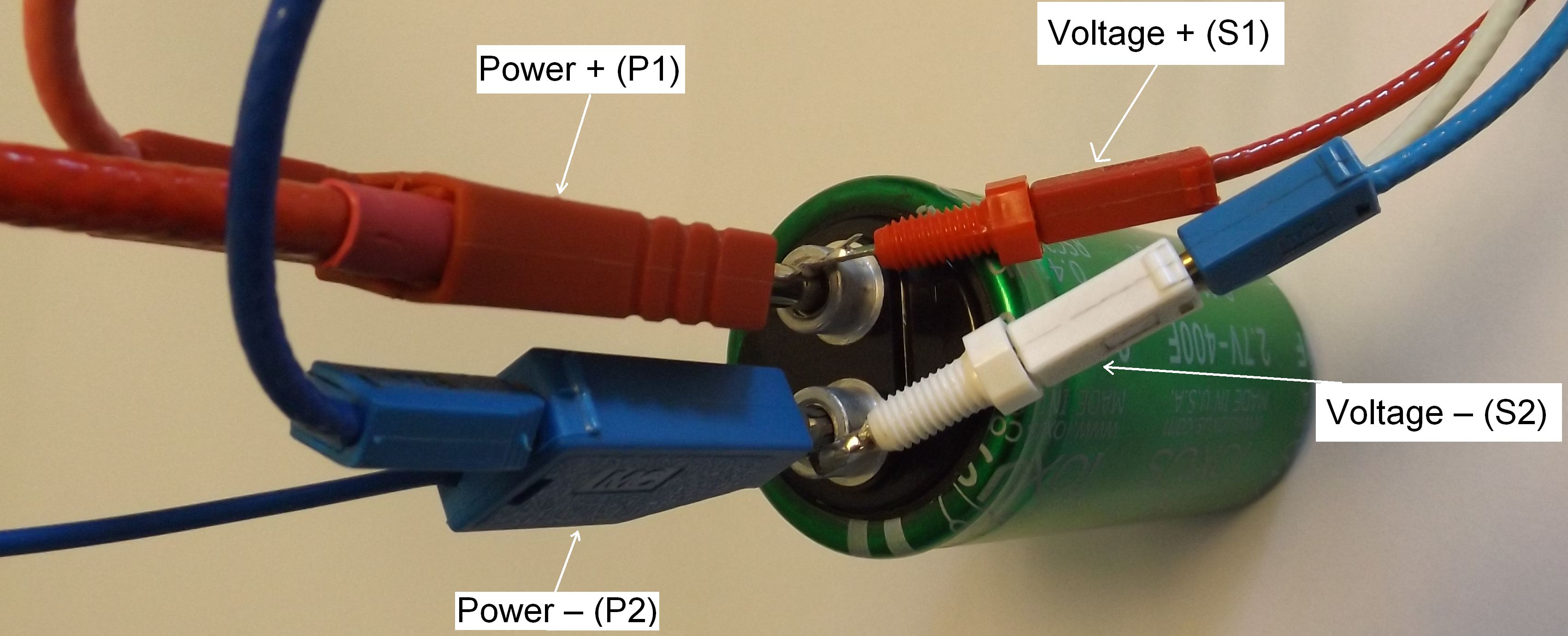
The figure below shows the setup used for the charge and discharge of the SC400.

Figure 1:  Example of setup for SC400 testing.

Results

E VS. Time Curves

Figures 2a and 2b show the obtained voltage profiles for the two tested supercapacitors. The charge and discharge were performed at the constant current of +/- 1 A for the SC22 and +/-8 A for the SC400.

Figure 2a: Voltage profiles for SC22.

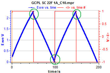
Figure 2b: Voltage profiles for SC400.

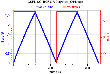
The beginning of each charge and discharge sequence on the SC22 voltage profile (Fig. 2a) displays a voltage drop (iR drop). This voltage drop corresponds to an important internal resistance. However, no significant IR drop was observed in the Fig. 2b indicating a low internal resistance for the SC400 supercapacitor. The internal resistance is discussed in the paragraph III-5.

The supercapacitor characteristics were calculated by processing the charge-discharge data using “Capacity & Energy per Cycle or Sequence” analysis tool. This tool is available in the supercapacitor section of Analysis tools menu of EC-Lab^®.

Figure 3: “Capacity & Energy per Cycle or Sequence” window.

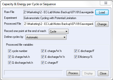
As shown in Fig. 3, the “Capacity & Energy per Cycle or Sequence” tool allows an EC-Lab^® user to calculate either for charge and discharge processes the capacity Q/mA.h, the capacitance C/F and the coulombic efficiency/%. These parameters are calculated as follows:

• Capacity: Q= I.Δt where I is the applied charge/discharge current and Δt is the charge/discharge duration.
• Capacitance C is calculated using the formula C =Q_ch/disch/ΔE_we, where Q_ch/disch is the total charge stored or released by the supercapacitor. ΔE_we is the voltage difference between the initial and final potential either on charging or discharging process.
• Coulombic efficiency is the ratio (Q_disch/Q_ch).100. As the charge and discharge were performed at the same current rate the coulombic efficiency is equal to (Δt_disch/Δt_ch)_.100 [4, 5] where Δt_disch and Δt_ch are the discharge and charge time, respectively.

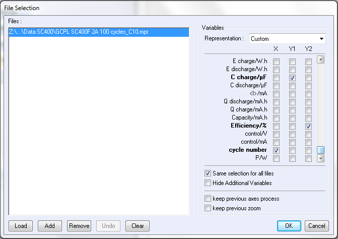
Once the charge-discharge data file is processed, the user can have access to the value of all the parameters mentioned above. In case of a charge-discharge cycling test, the user can also determine the parameters evolution vs. time (or vs. cycle number, voltage,…) using the following file selection window (Fig. 4).

Figure 4: File selection window.

Capacity Measurement

The capacity expresses the total charge stored or released by the capacitor during a full charge-discharge process. It can be displayed for each charge and discharge sequence and also for each cycle (1 charge+1 discharge).

Figs. 5a and 5b show the evolution (vs. cycle number) of the measured capacity Q_ch & Q_disch during charge and discharge of the two tested supercapacitors cycled 100 times using a galvanostatic charge-discharge protocol with current rates of 8 A and 2 A.

Figure 5a: Capacity vs. cycle number for the SC400.

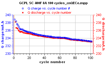
Figure 5b: Capacity vs. cycle number for the SC22.

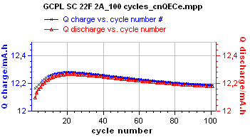
The measured capacities at the cycle 1 are around 239.0 mAh and 12.1 mAh respectively for the SC400 & SC22. These values decrease slightly with growing cycle number.

Capacitance Measurement

Capacitance is the main characteristic of a supercapacitor. It expresses the ability of a supercapacitor to store electrical energy.

The values of capacitance obtained for the cycle 1 and for SC400 and SC22 are 392 F and 21 F respectively. These results are in agree-ment with the nominal capacitance values provided by manufacturers which are 400 F + 10%/- 5% and 22 F +/- 30%.

The two supercapacitors have been cycled over 100 times at charge/discharge rates of 8 A and 2 A respectively. The evolutions of the capacitances vs. cycle number are presented in the Fig. 6a and 6b below.

Figure 6a: Charge & discharge Capacitance vs. cycle number for the SC400 supercapacitor.

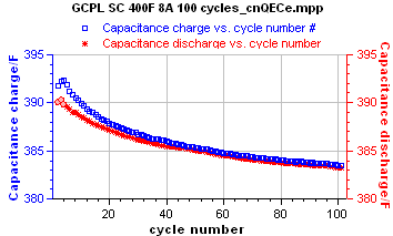
Figure 6b: Charge & discharge Capacitance vs. cycle number for the SC22 supercapacitor.

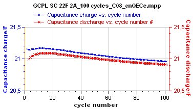
The Fig. 6a and 6b show a shallow, constant decrease of capacitance upon cycling. The measured capacitance decrease reached around 2% of the initial measured value after 100 cycles.

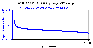
In order to check the evolution of the measured capacitance for a long time a long-term cycling test (10,000 cycles) was performed on the two supercapacitors. The result shows a capacitance decrease during the initial hundred cycles. The decrease becomes slightly smaller with growing cycle number. The Fig. 7 shows the obtained capacitance vs. cycle plot for the SC22.

Figure 7: Capacitance vs. cycle number for a long-term cycling test of the SC22.

The capacitance was also calculated for the same charge-discharge rates using the classical equation below:

$$C(F)= \frac{I_\text{ch/disch}}{|\text{Slope of }E_\text{WE} \; vs. \; t|}$$

Where I_ch/disch is the charge or discharge current and abs (slope E_we vs. t) is the absolute value of the slope of E_we vs. time curve. The obtained values of capacitance are 387 F and 21 F for SC400 and SC22 respectively.

Contrary to the classical method which leads to large errors for low rates of charge-/discharge where the E_we vs. t curve is not perfectly linear, the “Capacity and Energy per Cycle or Sequence” analysis tool provide an accurate capacitance value for low charge/discharge rates.

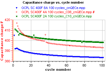
The SC400 was cycled over 100 times at charge/discharge rate of 8 A, 4 A and 2 A. The Fig. 8 shows a decrease of the measured capacitance with the increase of the cycling current. The capacitance decrease with incr-easing charge-discharge current was already observed in numerous studies [11, 12].

The obtained values of capacitance are more accurate and close to the nominal capacitance for the low current rates.

Figure 8: Capacitance vs. cycle number for the SC400 with three current rates (green 2 A, red 4 A, blue 8 A).

Efficiency Measurements

Once the charge-discharge data is processed by the analysis tool the coulombic efficiency vs. cycle number can be automatically plotted. Figures 9a and 9b show the obtained graphs.

Figure 9a: Coulombic efficiency vs. cycle number for SC400.

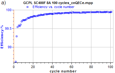
Figure 9b: Coulombic efficiency vs. cycle number for SC22.

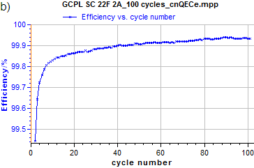
As shown in the Fig. 9a and 9b, both tested supercapacitors display a coulombic efficiency higher than 99%.

ESR Measurement

The internal resistance or Equivalent Series Resistance of a supercapacitor is classically determined from the charge-discharge curves using the voltage drop at the beginning of the discharge curve. The internal resistance which is also referred to as the Equivalent Series Resistance (ESR) [6] is due to the resistance of terminal leads, electrolyte, separator and current collectors.

Two different methods have been used to determine the internal resistance of each supercapacitor: EIS method and galvanostatic polarization method.

1. EIS method

Impedance measurements at rated voltage were performed on each supercapacitor in the frequency range 200 kHz-100 mHz with a voltage amplitude of 10 mV.

Figs. 10a and 10b present the Nyquist diagrams for the two capacitors.

Figure 10a: Nyquist diagram of SC400 supercapacitor.

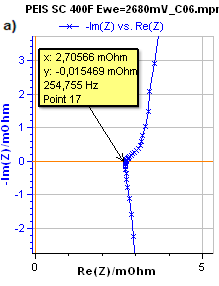
Figure 10b: Nyquist diagram of SC22 supercapacitor.

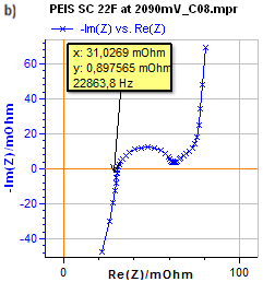
In the high-frequency range, the Nyquist diagrams show inductive behavior and then, intersect the real axis at approximately Re(Z)= 2.7 mΩ and 31.0 mΩ for  SC400 and SC22, respectively. These values, also obtained by fitting the two diagrams, correspond to internal resistance ESR [6-8] of the two supercapacitors.

Fig. 10c shows the fitted Nyquist diagram for the SC22.

Figure 10c: Fitting of the Nyquist diagram of SC22.

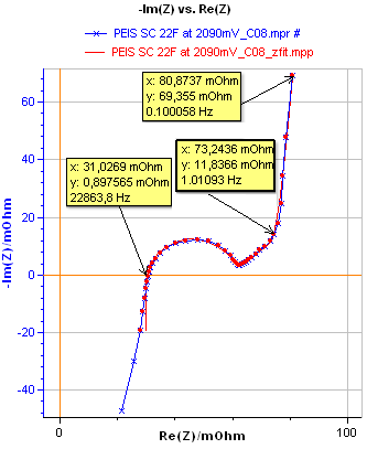
The equivalent circuit used to model the Nyquist diagram of the SC22 is shown below

Figure 11: Equivalent circuit used for Nyquist diagram of SC22 supercapacitor.

Where R1 is the internal resistance (ESR) of SC22, L1 inductance due to the wiring setup. R2 and Q2 were used to fit the semicircle at high frequency. R2 and Q2 are the charge transfer resistance and the CPE corresponding to the charge transfer resistance in parallel with the double layer capacitance. Ma₃ is the Modified restricted diffusion element. Indeed, at low frequencies (lower than 1 Hz) Fig 10c shows a typical modified restricted diffusion behavior. Thus the “Modified restricted diffusion element” Ma element available in Z Fit library of EC-Lab^® was used for modeling this kind of diffusion. The impedance expression of Ma is as follows [9].

$$Z_\text{d} =R_\text{d}(j \omega \tau)^{-\alpha/2} \text{coth}(j \omega \tau)^{\alpha/2}$$

Where R_d is the diffusion resistance, ω is the angular frequency, τ is the time constant and α a real parameter equal to 0.94.

The values of the ESR obtained from the fit of the Nyquist diagrams are close to those provided by the supercapacitors manu-facturers (respectively ESR (SC400) = 2.0 mΩ & ESR (SC22) < 100 mΩ).

As the internal resistance values of supercapacitors are very low the use of the four terminal connection points is strongly recommended to minimize the effect of the wiring on the value of ESR.

Figure 12: Four terminal connection points performed with SP-300/10A system.

1. Galvanostatic polarization method

The internal resistances of the two super-capacitors were also estimated from the vol-tage drop (iR_drop) divided by the total change in current applied (2. I_ch/disch) using the following equation [10]:

ESR =iR_drop/2.I_ch/disch

The Fig. 13 shows one charge discharge cycle performed on SC400 supercapacitor with a zoom on the voltage drop.

Figure 13: IR drop at the initiation of a 8A discharge curve of SC400 supercapacitor.

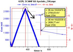
As can be seen from Fig. 13, the voltage drop observed during switching from charge to discharge regime is ΔE_we= 43 mV. This voltage was divided by twice the applied current. The obtained ESR value is ESR = 2.7 mΩ.

Conclusion

Galvanostatic polarization method is a fast and easy method for the determination of supercapacitor characteristics. The “Capacity and Energy per Cycle or Sequence“ is a powerful tool for the calculation of the supercapacitor parameters (capacity, energy, capacitance & efficiency). These parameters are quickly determined by processing the galvanostatic charge-discharge data using the analysis tool. The obtained parameters for the two supercapacitors clearly showed a good agreement with the characteristics values provided by the manufacturers. Based on an analytical approach, the “Capacity & Energy per Cycle or Sequence” tool provides accurate values of supercapacitors parameters.

Data files can be found in :

C:\Users\xxx\Documents\EC-Lab\Data\Samples\Supercapacitor\AN51 _GCPL SC X

References

1) M. D. Stoller, R.S. Ruoff, Energy Environ. Sci., 3 (2010) 1294.
2) Application Note #33 “Supercapacitors investigations – Part I: Charge/discharge cycling”
3) Application Note #34 ”Supercapacitors investigations – Part II: Time constant determination”
4) C. T. Hsieh, Y.W. Chou, W.Y. Chen, J. Solid State Chem., 12 (2008) 663.
5) H. Yu, Q. Tang, J. Wu, Y. Lin, L. Fan, M. Huang, J. Lin, Y. Li, F. Yu, J. Power Sources 206 (2012) 463.
6) K.H. An, K.K. Jeon, J.K. Heo, S.C. Lim, D.J. Bae, Y.H. Leez, J. Electrochem. Soc., 149 (2002) A1062.
7) X. Liu, P.G. Pickup, J. Power Sources 176 (2008) 410.
8) R. Kotz, M. Hahna, R. Gallay, J. Power Sources 154 (2006) 550.
9) T. Hang, D. Mukoyama, H. Nara, T. Yokoshima, T. Momma, M. Li, T. Osaka, J. Power Sources 256 (2014) 226.
10) G. Ma, J. Li, K. Sun, H. Peng, J. Mu, Z. Lei, J. Power Sources 256 (2014) 281.
11) Y. Fu, J. Song, Y. Zhu, C. Cao, J. Power Sources 262 (2014) 344.
12) Y. Bai, R.B. Rakhi, W. Chen, H.N. Alshareef, J. Power Sources 233 (2013) 313.