

CV Sim: Simulation of the simple redox reaction (E) – Part I: The effect of scan rate Kinetics – Application Note 41-1
Latest updated: January 31, 2024Abstract
In this note, the effect of the voltage scan rate on the shapes of the I vs. E curves is described for reversible and irreversible reactions. As a reminder, to investigate a redox system under standard conditions, one needs to make several CVs with different scan rates and analyze the evolution of peak current Ip and peak potential Ep with the scan rate. If Ep is invariant and |Ip| is proportional to √ν, it means the reaction is reversible (high k°). The diffusion coefficient DA and the standard potential E° of the reaction can be determined. If Ep varies with log(ν) and |Ip| is proportional to √ν, it means the reaction is irreversible (low k°). The symmetry factor αr and the standard constant k° of the reaction can be determined.
In a real experiment, the ohmic drop and the double layer capacitance current are not negligible. They must be taken into account, which is possible with CVSim and is the subject of the second part of this application note.
Introduction
CVSim is a powerful tool implemented in EC-Lab® that allows the user to simulate current vs. potential curves resulting from a voltammetry experiment. A vast array of parameters can be modified, making CVSim a very accessible tool to understand what kind of information can be obtained by voltammetry on the studied electrochemical system. In this application note, the simplest conditions are used. The reaction is a simple redox reaction:
$$A+ne\leftrightarrow\ B \tag{1}$$
where $A$ is the oxidizing species, $B$ the reducing species, $n$ the number of electrons, only the oxidizing species is present in the solution. Only a linear voltammetry (one single scan) is performed.
Definitions
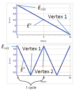
We define the linear voltammetry as a forward potential scan performed from the initial potential $E_\text{init}$ to the first vertex potential (either higher or lower than the standard potential). The cyclic voltammetry is a potential scan starting at $E_\text{init}$, going forward to the first vertex potential and backward to a second vertex potential. A cycle is defined as a potential scan from the first vertex potential to the second and back to the first (Figs. 1, top and bottom).

Figure 1: Potential vs time during top) linear voltammetry and bottom) cyclic voltammetry (Einit = 0.7 V, E° = 0.2 V, Vertex 1 = -0.3 V, Vertex 2 = 0.7 V)
The peak current $I_\text{p}$ is defined as the maximum current obtained during the forward linear potential scan. The corresponding potential is named the peak potential $E_\text{p}$ (Fig. 2). It is worth noting that the oxidizing species concentration $C_\text{a}$ at the electrode interface tends toward 0 at a potential lower than $E_\text{p}$. At $E_\text{p}$ the interfacial concentration is around 20% of the initial concentration. The interfacial concentration at the current peak can be easily calculated [1].

Figure 2: The peak current Ip and peak potential Ep.

Description of CVSim
The CVSim tool is available in the Analysis tab of the main menu of EC-Lab® (or EC-Lab Express®) (Fig. 3)

Figure 3: Where to find the CVSim tool in EC-Lab®.

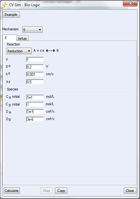
Once CVSim is open, it is possible to choose which reaction is simulated: from one to five step redox reaction (E to EEEEE), involving from one to 6 species (Fig. 4a). EC, CE reactions are also available (not shown in Fig. 4a). E stands for electron transfer and C for chemical reaction. It is also possible to choose an example from a selection of preset parameters, often referring to conditions used in publications.
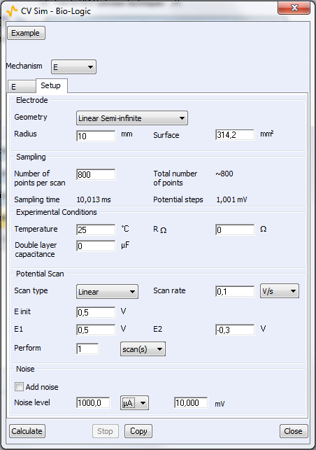
Two parameters windows are available: the first one is related to the reaction itself (Fig. 4a) and the second window is related to the experimental parameters (Fig. 4b). For a classic CV from $E_\text{init}$ to Vertex 1 (E1) and then Vertex 2 (E2), the number of scans is 2. For a linear scan, the number of scans is 1.


Figure 4: The parameters windows related to bottom) the reaction and top) the experimental setup.
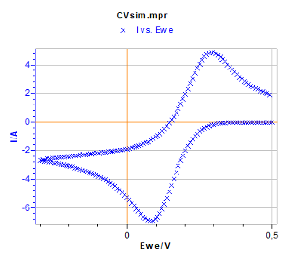
By clicking Calculate, the simulated I-E curve corresponding to the parameters set in the two former windows can be obtained (Fig. 5). The corresponding data file named CVsim.mpr is located in the following folder: C:\Users\your.name\Documents\EC-Lab\Data.
Each time a new simulation is performed the “CVsim.mpr” file is replaced. In order to keep the data, the user must change the name of this file.

Figure 5: Cyclic voltammetry corresponding to the default parameters set in Figs. 2a) and 2b).
Kinetic study of the (E) redox reaction using variable scan rates
The reversible (or Nernstian) behaviour
In this example, the parameters are the following:
- $k°$ = 10 cm·s-1
- $\alpha_\text{f}$ = 0.5
- $E°$ = 0.2 V
- Initial $C_\text{A}$: 10-5 mol·cm-3 (10-2 mol·L-1) and initial $C_\text{B}$ : 0 mol·L-1
- $D_\text{A}$ = $D_\text{B}$ = 10-6 cm2·s-1
- $A$ = 0.03142 cm2 with linear semi-infinite diffusion
- $E_\text{init}$ = $E°$ + 0.3 V
- $E1$ = – 0.3 V
- $E2$ = 0.5 V
Note that $k°$ has been chosen high enough to ensure that the reaction has a reversible behaviour for scan rates that are commonly experimentally used.
The first used scan rate is 10 mV·s-1, that we multiply each time by 4 to have the next one: 40, 160, 640 and so on…
The results are given in Fig. 6. For each curve the values of the peak voltages and peak currents are noted. We can see that the peak current $I_\text{p}$ increases in absolute value as the scan rate increases while the peak voltage $E_\text{p}$ remains relatively constant. The latter shows that the reaction is not irreversible.

Figure 6: I vs. E curves with increasing scan rates: Red curve: 10 V·s-1; Green curve: 40 V·s-1; Purple curve: 160 V·s-1; Pink curve: 640 V·s-1; Blue curve: 2,560 V·s-1 with k° = 10 cm·s-1.
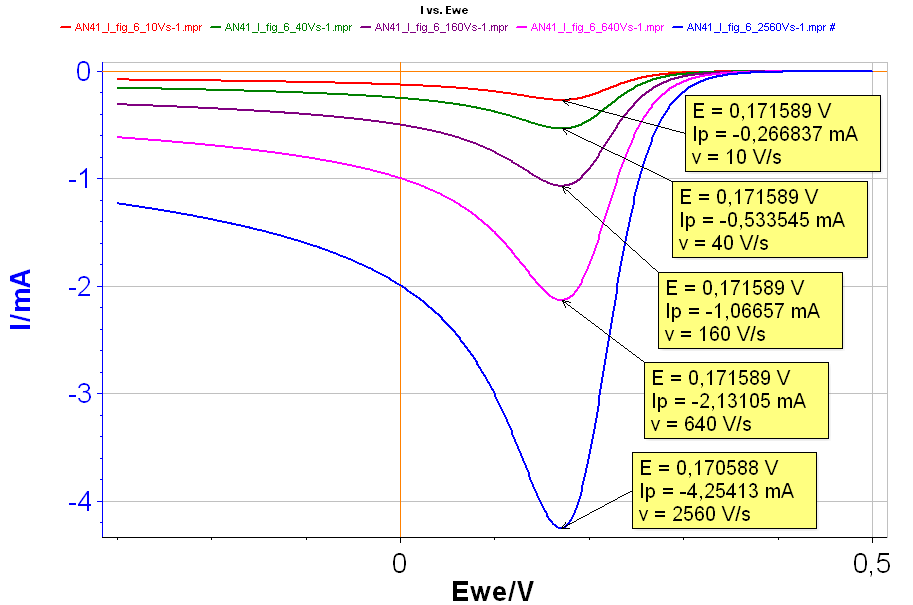
From the curves in Fig. 6, it can be seen that $I_\text{p}$ is proportional to $\nu$1/2, with $\nu$ the scan rate: as $\nu$ is multiplied by 4, $I_\text{p}$ is multiplied by 2. This is a proof that the reaction is reversible. Plotting $I_\text{p}$ as a function of $\nu$1/2 gives the curve shown in Fig. 7, where it can be seen that there is a linear relationship between $I_\text{p}$ and $\nu$1/2.

Figure 7 : |Ip| (mA) vs. ν1/2 (V1/2·s–1/2).

The relationship between $I_\text{p}$ and $\nu$ is given by Bard and Faulkner [2, p. 231]:
$$I_p = −0.446AnFC^*_\text{A} \sqrt{nf \nu D_\text{A}}; f = F/RT \tag{2}$$
With F, the Faraday constant (96485 C·mol-1), R the ideal gas constant (8.314 J·K-1·mol-1), T the ambient temperature (298 K), $C^*_\text{A}$ the bulk concentration of species A in mol·cm-3, n the number of exchanged electrons, $D_\text{A}$ the diffusion coefficient of species A in cm²·s-1 and $\nu$ the scan rate in V·s-1.
The slope p of the curve shown in Fig. 7 is:
$$p = -0.446AnFC^*_\text{A} \sqrt{nfD_\text{A}} \tag{3}$$
which can be used to determine the diffusion coefficient of species A in the electrolyte considered:
$$D_A = \left(\frac{p}{−0.446AnFC^*_\text{A} \sqrt{nf}}\right)^2 \tag{4}$$
Using the slope shown in Fig. 7, the parameters given above and Eq. 4, we obtain for $D_\text{A}$, a value of 0.989 10-6 cm2·s-1, which is quite close to the value used in the simulation.
The factor -0.446 of Eq. 2, only holds for reversible systems. Equation 2 can be rearranged, and by replacing -0.446 by M, it gives:
$$M = \frac{-I_p}{AnFC^°_\text{A} \sqrt{nf \nu D_\text{A}}} \tag{5}$$
This means that the reversible behaviour of the reaction can be “tested” for each scan rate: if M = -0.446, it means the reaction has a reversible behaviour. Table I shows the calculated M values for each scan rate:
Table I: M values as a function of the scan rate v.
| ν (V·s-1) | M |
| 10 | 0.4460 |
| 40 | 0.4459 |
| 160 | 0.4457 |
| 640 | 0.4453 |
| 2560 | 0.4444 |
As the scan rate increases, the value of the factor M moves away from the theoretical value of -0.446. As the scan rate increases, the behaviour of the reaction is less and less reversible.
This shows that reversibility and irreversibility are not only related to the value of $k°$ but also to experimental conditions such as the scan rate.
The peak potential $E_\text{p}$ can help in determining the standard potential $E°$ of the reaction:
$$E^° = E_p + \frac{1}{2nf}\text{ln}\frac{D_\text{A}}{D_\text{B}}+\frac{1.109}{nf} \tag{6}$$
and
$$E^° = E_p + \frac{1.109}{nf} \tag{7}$$
if $D_\text{A}$ = $D_\text{B}$.
The irreversible behaviour
We use the same parameters as before, except $k°$, that we set at 0.001 cm·s-1. Choosing a small reaction rate constant, for which the kinetics of the reaction can be considered sluggish, ensures to have an irreversible behaviour of the reaction for commonly used scan rates.
The same scan rates as for Fig. 6 are used to plot the curves shown in Fig. 7.

Figure 8: I vs. E with increasing scan rates: Red curve: 10 V·s-1; Green curve: 40 V·s-1; Purple curve: 160 V·s-1; Pink curve: 640 V·s-1; Blue curve: 2,560 V·s-1 with k° = 0.001 cm·s-1.
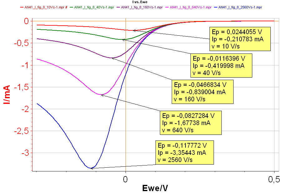
It can be seen in Fig. 8 that both $I_\text{p}$ and $E_\text{p}$ are changing with the scan rates, which shows that the behaviour of the reaction is not reversible. The higher the scan rate is, the higher $|I_\text{p}|$ and the lower $E_\text{p}$ are, in the case of a reduction reaction.
If we plot $E_\text{p}$ vs. ln($\nu$), it can be seen that there is a linear relationship, which shows that the reaction has an irreversible behaviour (Fig. 9).

Figure 9: Ep (V) vs. ln(v) (V/s) for an irreversible reaction.

For an irreversible system, or a reaction with an irreversible behaviour, the relationships between the peak current and the peak potential with scan rates are given by Bard et al. [1, p. 236]:
$$I_p = -0.496AnFC^*_\text{A} \sqrt{\alpha_\text{r}nf \nu D_\text{A}}; f=F/RT \tag{8}$$
$$E_p = E^° + \frac{1}{\alpha_\text{r}nf} \left(-0.178 + \text{ln}\frac{k^°}{\sqrt{\alpha_\text{r}nf \nu D_\text{A}}}\right) \tag{9}$$
All parameters have the same meaning as in Eq. 2 and $\alpha_\text{r} = \alpha_\text{f}$. Eq. 8 can be used to obtain the symmetry factor $\alpha_\text{r}$, as it can be written as an affine law:
$$E_p = a \text{ln} \nu + E_\text{oo} \tag{10}$$
With $E_\text{oo}$ the ordinate at the origin of the $E_\text{p}$ vs. ln($\nu$) curve and $a$ its slope.
$$a = – \frac{1}{2\alpha_\text{r}nf} =\!\Rightarrow \alpha_\text{r} = – \frac{1}{2anf}\tag{11}$$
Using the slope $a$, we can directly get the symmetry factor $\alpha_\text{r}$. Using the results shown in Fig. 9, we obtain a symmetry factor of 0.5008, very close from the value used in the simulation.
If we plot $I_\text{p}$ as a function of $\nu$1/2, we have the curve shown in Fig. 10.

Figure 10: Ip (A) vs. ν1/2 ((V·s-1)1/2) for an irreversible reaction.
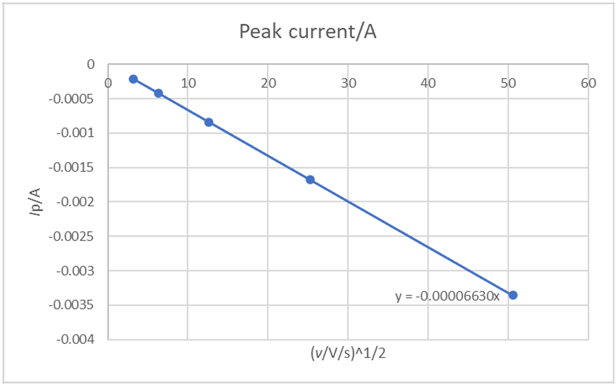
It can be seen in Fig. 9 that there is a linear relationship between $I_\text{p}$ and $\nu$1/2 as expected by Eq. 8.
The slope of this curve can be used to obtain the diffusion coefficient:
$$I_\text{p} = b \sqrt{\nu} \tag{12}$$
With
$$b=-0.496AnFC^*_\text{A} \sqrt{\alpha_\text{r}nf D_\text{A}} =\!\Rightarrow D_\text{A} \tag{13}$$
If we use the value of the symmetry factor obtained before, we have $D_\text{A}$ = 9.96 10-7 cm2·s-1, which is very close to the value used in the simulation.
Finally, with $E_\text{oo}$¸ we can obtain the standard reaction rate constant as:
$$E_\text{oo} = E^° + \frac{1}{\alpha_\text{r}nf}\left(-0.78 + \text{ln} \frac{k^°}{\sqrt{\alpha_\text{r}nfD_\text{A}}}\right) =\!\Rightarrow \\k^° = \text{exp} \left(\alpha_\text{r}nf\left(E_\text{oo}-E^° \right) + 0.78 + \text{ln}\sqrt{\alpha_\text{r}nf D_\text{A}}\right) \tag{14}$$
Using $E°$ = 0.2 V, it gives $k°$ = 9.86·10-4 cm·s-1, which is very close to the value used in the simulation.
Finally, Eq. 8 and the value of -0.496 for the multiplying coefficient is valid only for a totally irreversible reaction behaviour. For each point of the curve shown in Fig. 10, we can recalculate the value of this factor N using the following equation, similarly to what was done in the case of the reversible behaviour:
$$N = \frac{-I_\text{p}}{AnFC^*_\text{A} \sqrt{\alpha_\text{r}nf \nu D_\text{A}}} \tag{15}$$
Table 2: N values as a function of the scan rate $\nu$ for the reversible behaviour.
| ν (V·s-1) | N |
| 10 | -0.4983 |
| 40 | -0.4964 |
| 160 | -0.4959 |
| 640 | -0.4957 |
| 2560 | -0.4956 |
It can be seen that the factor N is quite far from the theoretical value for the lowest scan rate used here i.e., 10 V·s-1. This shows that as we decrease the scan rate, the reaction behaviour tends to become less irreversible. If we use a sufficiently low scan rate, the reaction behaviour could be reversible.
Again, the reversible/irreversible behaviour of a reaction depends on the standard reaction rate constant, which quantifies the electron transfer kinetics and experimental factors affecting mass transport such as in our case scan rate, but it could also be rotation rate in the case of an RDE.
Conclusion
Using CVSim, it was presented how performing CVs at various scanning rates can lead to extremely useful information on the studied redox reaction. It was demonstrated in the case of the simple E redox reaction. The appendix summarizes the various conclusions of this application note and gives some guidelines to interpret the results step by step. In a real experiment, there is an ohmic drop and the double layer capacitance current is not negligible. They must be considered, which is possible with CVSim and is the subject of the second part of this application note.
References
- https://biologic.net/topics/cvsim-as-alearning-tool-ii-interfacial-concentrations/ (Accessed on 6/2022)
- A. J. Bard, L. R. Faulkner, Electrochemical Methods: Fundamentals and Applications, Wiley, Hoboken, (2001).
Revised in 06/2022
Scientific articles are regularly added to BioLogic’s Learning Center:
https://biologic.net/topics/ To access all BioLogic’s application notes, technical notes and white papers click on Documentation: https://biologic.net/documents/
Appendix
Added in 04/2023


