

The modified inductance element $L_\text a$ Battery – Application Note 42
Latest updated: January 31, 2024Abstract
A Constant Phase Element (CPE) can be physically interpreted as an effect of the surface roughness of the sample, leading to a heterogeneity of the capacitance. On the other hand, the modified inductance, La, can be used to represent the presence of an unusual inductance in the Nyquist diagram. The expression of the impedance of an inductance is $Z_\text L (f)=Lj2πf$. The expression of the impedance of the modified inductance $L_\text a$ is $Z_{\text L_\text a} (f)=L_\text a (j2πf)^a$ with $L$ and $L_\text a$ the value of the inductance in H and of the modified inductance in H·s(a-1), respectively, with 0<a≤1.
This application note introduces a few practical cases for which the modified inductance component can lead to a much better fit of impedance data. The new element $L_\text a$ is a modified inductance element. It can be used to fit impedance characteristics related to either an unusual connection inductance at high frequencies (i.e. mostly visible in batteries or a heterogeneous adsorption mechanism) or at low frequencies (i.e. mostly visible in corrosion).
Introduction
It is convenient to use a Constant Phase Element (CPE) instead of a capacitor when for instance the Nyquist diagram of the impedance of a system shows a semi-circle whose center is located below the Real axis, instead of on the Real axis.
The difference between a capacitor $C$ and a CPE $Q$ is that the expression of the impedance of a CPE contains an additional parameter a:
$$Z_\text Q (f)=\frac{1}{Q(j2πf)^a} \tag{1}$$
whereas the expression of the impedance of the capacitor is:
$$Z_\text C (f)=\frac{1}{Cj2πf} \tag{2}$$
with $C$ and $Q$ the value of the capacitor in F and of the CPE in F·s(a-1) with 0 < a ≤ 1. It is important to note that $Z_\text Q (f) = Z_\text C (f)$ for a = 1. A CPE is physically interpreted as an effect of the surface roughness of the sample, leading to an heterogeneity of the capacitance.
Analogously, the modified inductance $L_\text a$ can be used to represent the presence of an unusual inductance in the Nyquist diagram. The expression of the impedance of an inductance is:
$$Z_\text L (f)=Lj2πf \tag{3}$$
The expression of the impedance of the modified inductance $L_\text a$ is:
$$Z_{\text L_\text a} (f)=L_\text a (j2πf)^a \tag{4}$$
with $L$ and $L_\text a$ the value of the inductance in H and of the modified inductance in H·s(a-1), respectively, with 0 < a ≤ 1. Again, $Z_{\text L_\text a} (f)=Z_{\text L} (f)$ for a = 1.
This application note introduces a few practical examples for which the modified inductance component can lead to a much better fit of impedance data.
High-frequency inductance in Li-Ion batteries
Figure 1 shows the Nyquist impedance diagram of an LiPF6 Li-ion battery with a capacity of 60 Ah and a nominal voltage of 3.2 V. An inductive behaviour can be seen at high frequencies (f > 22 Hz), most likely due to the connection cables to the battery. This behaviour is more visible in cells with low apparent resistance such as batteries. As shown by the least square linear fit in Fig. 1, these high frequency data points are on a straight line that is not perpendicular to the x-axis. Consequently, this behaviour cannot be represented by a simple inductance.

Figure 1: Nyquist impedance diagram of an LiPF6 battery for frequencies ∈ [0.1 , 2000] Hz.
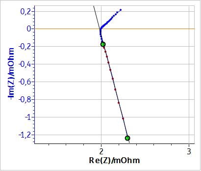
Figure 2 shows the equivalent circuit chosen to fit the data shown in Fig. 1.

Figure 2: Randles equivalent circuit with a modified inductance in series.
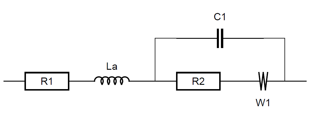
It is a Randles circuit with an inductance $L_\text a$ in series. The simple $L$ is a particular example of the inductance $L_\text a$. As stated above, if a = 1, $L_\text a$≡$L$. R1 is associated to the internal resistance of the battery, C1 to the double layer capacitance, R2 to the charge transfer resistance and W, the Warburg component, to the semi-infinite diffusion.
Figure 3 shows the fitting curve obtained using the equivalent circuit shown in Fig. 2 with a simple inductance. Fig. 4 shows the same results but with a modified inductance $L_\text a$. A comparison of the results of the two fitting, i.e. the values of the parameters and of $\chi^2$ (an estimation of the goodness of the fit [1]) are given in Table 1.

Figure 3: Fitting results of the impedance diagram in Fig. 1 using the equivalent circuit: L1+R1+C1/(R2+W1).
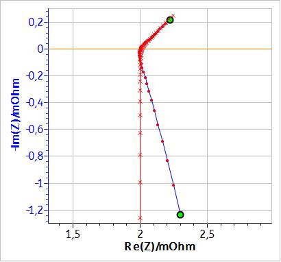
If, instead of an inductance $L$, a modified inductance $L_\text a$ is used as shown in Fig. 3, it is possible to fit the non-vertical high frequency part of the impedance. Fig. 4 shows the results of the fitting of the battery impedance in Fig. 1 using the modified inductance in series with a Randles equivalent circuit. In this case, $\chi^2$ is lower and hence better than the $\chi^2$ factor obtained with an equivalent circuit containing a simple inductance (cf. Table 1). Furthermore, in Table I, it can be seen that the values of C1, R2 and W1 are different, which shows that using a modified inductance leads to a better determination of the characteristic parameters of the system.

Figure 4: Fitting results of the graph in Fig. 1 using the equivalent circuit: La1+R1+C1/(R2+W1).
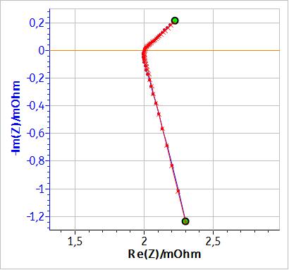
Table I: Values of the parameters for the equivalent circuits used in Fig. 3 and Fig. 4.
| Parameter | Using $L$ (Fig. 3) | Using $L_ \text a$ (Fig. 4) |
|---|---|---|
| L1 /µHs(a-1) | 0.14 | 0.48 |
| a1 | 1 | 0.84 |
| R1 /mΩ | 2 | 2 |
| C1 /F | 109 | 429 |
| R2 /µΩ | 14.3 | 50.3 |
| s1 /mΩ s-1/2 | 0.17 | 0.158 |
| $\chi^2$ | 0.53×10⁻⁶ | 2.67×10⁻⁹ |
Low frequency inductive behavior of a freely corroding metal
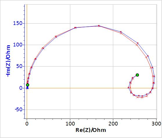
Another example of a system for which the component $L_\text a$ can be used is a metal corroding in an acidic solution. In this case, the reduction reaction is the proton reduction, which involves an adsorption step, following the Volmer-Heyrovský mechanism [2, 3]. Fig. 5 shows the impedance graph obtained on a partially painted Zn sample immersed in 0.5 mol·L-1 H2SO4 and the corresponding fitting curve using the equivalent circuit shown in Fig. 6.
In this equivalent circuit, Q1/R1 is associated to the larger semi-circle in Fig. 5 (possibly related to the coated part of the sample), Q2/R2 to the inductive semi-circle (related to an adsorption process at the rough metal surface) and Q3/R3 to the third semi-circle (also possibly related to the bare metal). The solution used in this example was not a perfect ionic conductor but its resistance of around 1 was considered negligible.
Another way to interpret the impedance diagram is to consider a Volmer-Heyrovský chemical desorption mechanism.

Figure 5: Blue: Nyquist diagram of the impedance of a partially coated Zn sample immersed in 0.5 mol L-1 H2SO4 for frequencies Î [10×10-3 , 200×103] Hz. Red: Fitting curve using Q1/(R1+Q2/R2+Q3/R3).
In the fitting results shown in Table II, the elements Q2/R2 correspond to the inductive loop and have negative values. It might be difficult for the user to handle and interpret negative values. It is then possible to use an equivalent circuit for which the elements have positive values. This can be done by replacing the circuit R1+Q2/R2 in Fig. 6 by R1/(R2+La2) as shown in Fig. 7.

Figure 6: Equivalent circuit used in Fig. 5.
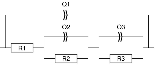
Table II: Values of the parameters for the equivalent circuits used in Fig. 5.
In Fig. 8, the blue curve shows the experimental data, the red curve, the fitting curve obtained using the equivalent circuit in Fig. 7 with a simple inductance (a2 = 1) and the green curve, the fitting curve obtained using the equivalent circuit in Fig. 7 with a modified inductance.
As can be seen in Table III, all the elements of the equivalent circuit have now positive values. In terms of choosing the best equivalent circuit, it seems the red curve fit less tightly to the real data than the green curve, which shows that the modified inductance increases the goodness of the fit (see inset of Fig. 8). This is confirmed by the values of the χ2 shown in Table 3.

Figure 7: Equivalent circuit used in Fig. 8.
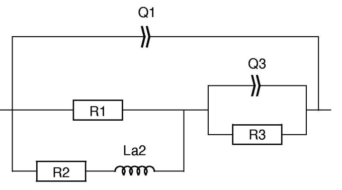

Figure 8: Blue: Nyquist diagram of the impedance of a partially coated Zn sample immersed in 0.5 mol·L-1 H2SO4.Fitting curve using Red : Q1/(R1/(R2+L2)+Q3/R3), Green : Q1/(R1/(R2+La2)+Q3/R3).
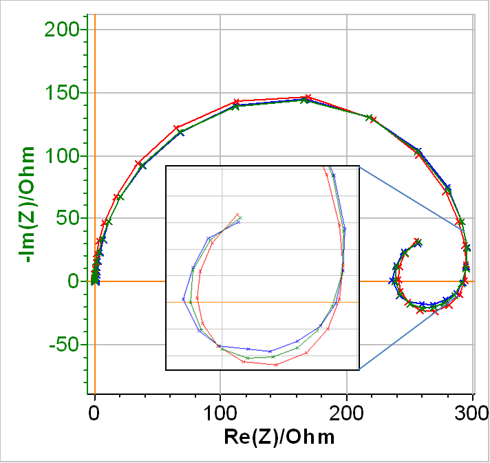
Table III: Values of the parameters for the equivalent circuits used in Fig. 8.
| Parameter | Fig. 5 Red |
|---|---|
| Q1 /µF s(a-1) | 65.5 |
| a1 | 0.982 |
| R1 /Ω | 298 |
| Q2 /F s(a-1) | -0.015 |
| a2 | 0.907 |
| R2 /Ω | -75.1 |
| Q3 /F s(a-1) | 0.168 |
| a3 | 0.826 |
| R3 /Ω | 122 |
| $\chi^2$ | 325 |
Conclusion
The new element $L_\text a$ is a modified inductance element. It can be used to fit impedance characteristics related to either an unusual connection inductance at high frequencies, mostly visible in batteries or a heterogeneous adsorption mechanism at low frequencies, mostly visible in corrosion.
References
1) EC-Lab User’s Manual p. 113
2) M. Keddam, Thèse, Paris, 1968, no. AO2192.
3) J.-P. Diard, P. Landaud, B. Le Gorrec, C. Montella, J. Electroanal. Chem., 255 (1988) 1.
Data files can be found in:
Fig. 1 : C:\Users\xxx\Documents\EC-Lab\Data\Samples\Battery\ AN42_battery
Fig. 5: C:\Users\xxx\Documents\EC-Lab\Data\Samples \Corrosion\AN42_coating
Appendix
- It is noteworthy that if the inductive loop in Fig. 5 could be fitted with an R/C instead of an R/Q (i.e. if a2 was equal to 1) then an R+L would be enough and R+La unnecessary.
- Furthermore, to widen the perception of what an equivalent circuit is, it is worth noting that ZQ(f) = ZLa(f) with aQ = –aLa and $Q = 1/L_\text a$, aQ being the a parameter for the element Q and aLa for the element La.
If we replace in Eq. 4, $a$ by -$a_\text Q$:
$$Z_{\text L_\text a} (f)=L_\text a (j2πf)^{(-a_\text Q)} \tag{5}$$
$$Z_{\text L_\text a} (f)=L_\text a/(j2πf)^{a_\text Q} \tag{6}$$
$$Z_{\text L_\text a} (f)=\frac{1}{Q(j2πf)^{a_\text Q}} \tag{7}$$
With $L_\text a=1/Q$
$$Z_{\text L_\text a} (f)=Z_\text Q (f) \tag{8}$$
Finally, the impedances of the $C$, $L$, $Q$ and $L_\text a$ elements are all particular forms of the general expression:
$$Z(f)=A(j2πf)^m \tag{9}$$
with $A$ the value of the component and m ∈ [-1,0[ È ]0,1].
If m = 0, then the impedance $Z$ is a simple resistance.
Revised in 11/2023


