

Distribution of Relaxation Times (DRT): an introduction Battery – Application Note 60
Latest updated: December 16, 2024Abstract
DRT is a tool that can be used to help interpreting impedance data. This note introduces the theoretical basis of this method as well as the advantages and limitations compared to direct electrical equivalent circuit modeling.
Introduction
Electrochemical Impedance Spectroscopy (EIS) is used to identify the physical characteristics of a system. The method is used to model the system using what is called an electrical equivalent circuit, where each element of the circuit is supposed to correspond to a physical characteristic of the system under study.
Fitting the impedance data using an electrical model gives access to the values of the elements and hence the physical characteristics, such as, for instance, time constants.
The choice of an electrical circuit requires prior knowledge of the impedance of each element and this is why impedance can be considered difficult to use at first.
DRT is an analysis method which turns impedance data that are a function of the frequency into a distribution of the time constants involved in the considered system.
DRT can be considered as a tool to help finding an equivalent circuit that should be used to fit impedance data.
In this note, we will present the main principles behind this analysis and show the various tools available to perform it.
We will then present the results to illustrate the advantages of this method as well as present some of its limitations.
Theory
Finite Voigt Circuit
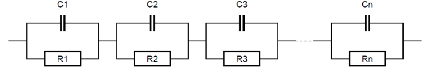
The Voigt circuit also called a measurement model [1] was used to fit impedance data. A Voigt circuit is composed of a series of N R/C circuits (Fig. 1), for which the impedance can be described:
$$Z(\omega)= \sum^N_{k=1}\frac{R_k}{1+i\omega\tau_k}\tag{1}$$
With $\tau_k = R_kC_k$

Figure 1: Voigt circuit. Sometimes a resistance in series is added.
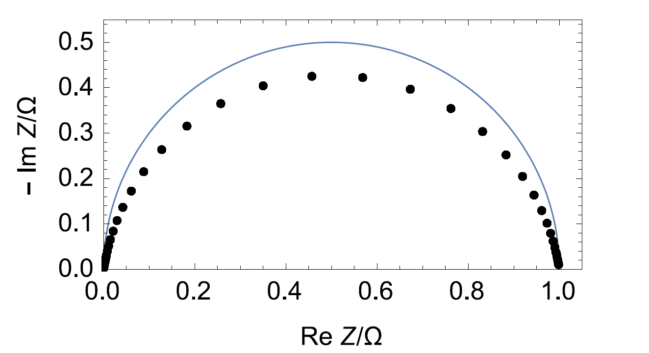
Let us consider an R/Q circuit, with R = 1 Ω,
α = 0.9, Q = 1 F.s-0.1, whose impedance diagram is shown in Fig. 2.

Figure 2: Nyquist impedance diagram of an R/Q circuit. The half circle in full line shows that the impedance data are not from a simple R/C circuit.
To fit these data, we can use as an equivalent circuit, a Voigt circuit with, for example, 17 R/C elements. For each Rk/Ck values, a time constant τk can be calculated. We can then plot Rk as a function of τk. The results are shown in Fig. 3.

Figure 3: Change of Rk vs. τk.
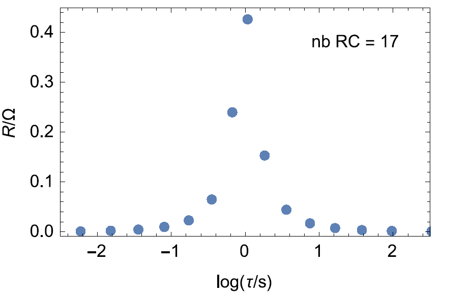
Figure 3 shows that Rk values loosely follow a Gaussian law. Furthermore, it can be verified that:
$$\sum^{17}_{k=1}R_k\approx 1\tag{2}$$
Infinite Voigt Circuit
Let us now consider a Voigt circuit with an infinite number of elements. It can also be used to fit the impedance data shown in Fig. 2 but instead of discrete values of Rk vs. τk, we have a continuous variation of R(τ), that is to say a distribution function.
The impedance of such a circuit can be described as [2]
$$Z(\omega)= \int^\infty_0\frac{G(\tau)}{1+i\omega\tau}d\tau\tag{3}$$
with G(τ) the distribution function of the relaxation times τ, which is characteristic of the system under test.
We can deduct from Eq. (3) that the unit of G is Ω.s-1.
If the analytical expression of the impedance of the system Z(ω) is known, we can use Eq. (3) to express the function G(τ).
For instance, for an R/Q circuit, we can have [2]:
$$G_{R/Q}(\tau)= \frac{R}{2\pi}\frac{\text{sin}((1-\alpha)\pi)}{\text{cosh}\left(\alpha\text{ln}\left(\frac{\tau}{\tau_{R/Q}}\right)\right)-\text{cos}((1-\alpha)\pi)}\tag{4}$$
With $\tau_{R/Q}=(RQ)^{1/\alpha}$.
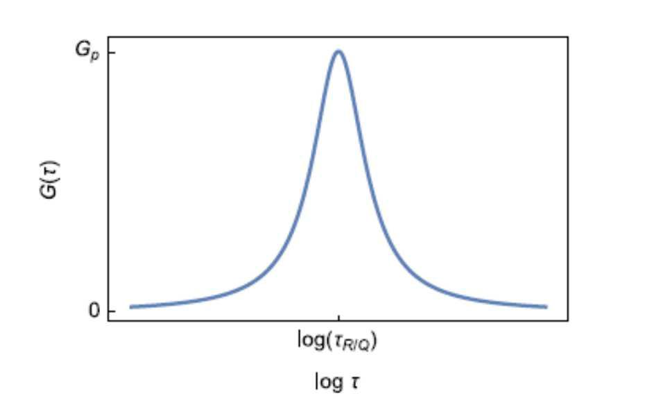
For a given set of parameters R, Q and α, we can plot G(τ). The abscissa of the peak gives the circuit time constant τR/Q and the G value at the peak is given by
$$\frac{dG}{d\tau}=0\implies G_p = \frac{R}{2\pi} \text{tan}\left(\frac{\alpha\pi}{2}\right)\tag{5}$$
Figure 4 shows the theoretical DRT of an R/Q circuit from Eq. (4):

Figure 4: Theoretical DRT of an R/Q circuit
Other expressions can be found in the literature for example, for a finite length diffusion impedance [3].
Experimental Data
The Problem
In the case of experimental data, the expression of the impedance is not known a priori. This means that Eq. (3) must be numerically solved using experimental impedance values to extract G(τ).
Eq. (3) is a Fredholm integral equation of the first kind, typical of an inverse problem. There are a few methods proposed in the literature to solve a Fredholm equation: Fourier transform [4], Maximum entropy [5], Bayesian approach [6], Ridge and lasso regression methods [7] and finally Tikhonov regularization [8], which is the one that will be evaluated and used in this paper.
One Solution
Several programs have been written by researchers to calculate DRT using Tikhonov regularization: FTIKREG [9] and DRTtools [2,10]. The latter is a MATLAB application, which was used to produce data shown in this note, that are compared with the results obtained using a theoretical expression of G(τ), available for an R/Q circuit and a series of two R/Q circuits.
Here is the method:
- Electrical circuits are chosen with various parameters.
- Z Sim, the simulation tool in EC-Lab®, is used to simulate and plot impedance data.
- These impedance data are used as inputs in the DRT tools used to provide an approximation of the DRT.
- For each circuit, the theoretical DRT is plotted using the theoretical expression of G(τ) (Eq. (3)).
- Both DRTs are compared.
The circuit that we are interested in is composed of two R/Q in series: R1/Q1+R2/Q2. Table I shows the parameters used for the three different circuits. Only the parameter Q2 changes.
Table I: Parameters for the R1/Q1 + R2/Q2 circuit
| 1 | 2 | 3 | |
|---|---|---|---|
| R1/Ω | 1 | ||
| Q1/F.s(α1-1) | 10-3 | ||
| α1 | 0.9 | ||
| R2/Ω | 1 | ||
| Q2/F.s(α2-1) | 10-3 | 0.3×10⁻³ | 0.1×10⁻³ |
| α2 | 0.9 | ||
Figure 5 shows the simulated impedance graph in the Nyquist plane of the three circuits described in Tab. I. ZSim from EC-Lab® was used.

Figure 5: Simulated impedance graph of the three circuits shown in Tab. I.
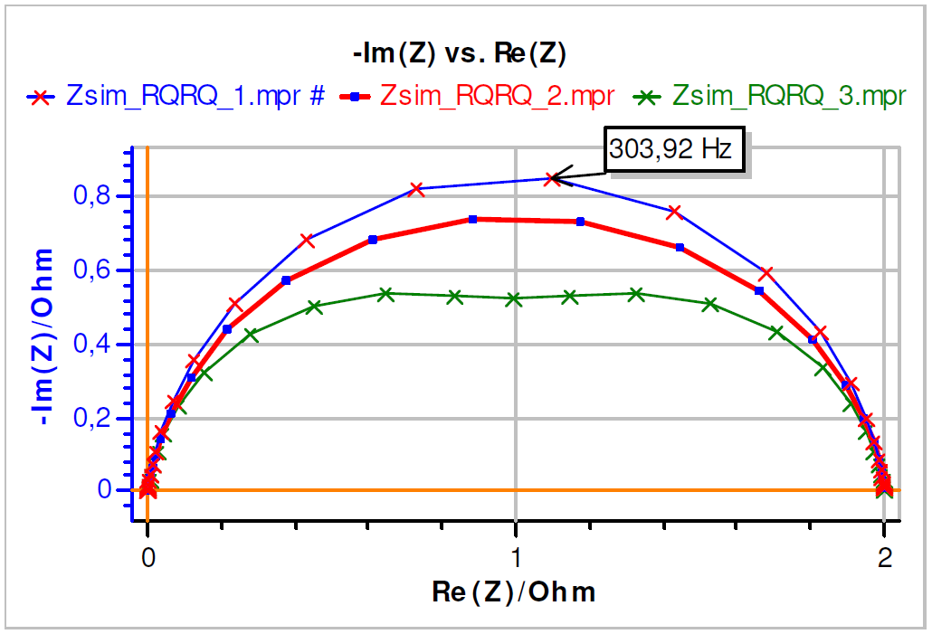
The graph corresponding to the first circuit consists of a single arc, which is to be expected since the R/Q elements have the same parameters and hence the same time constants.
The time constant can be determined using the characteristic frequency fc at the apex of the diagram, which is in Fig. 5: 304 Hz. We then have:
$$\tau=\frac{1}{2\pi f_c}\tag{6}$$
This gives τ = 4.6 x 10⁻⁴ s.
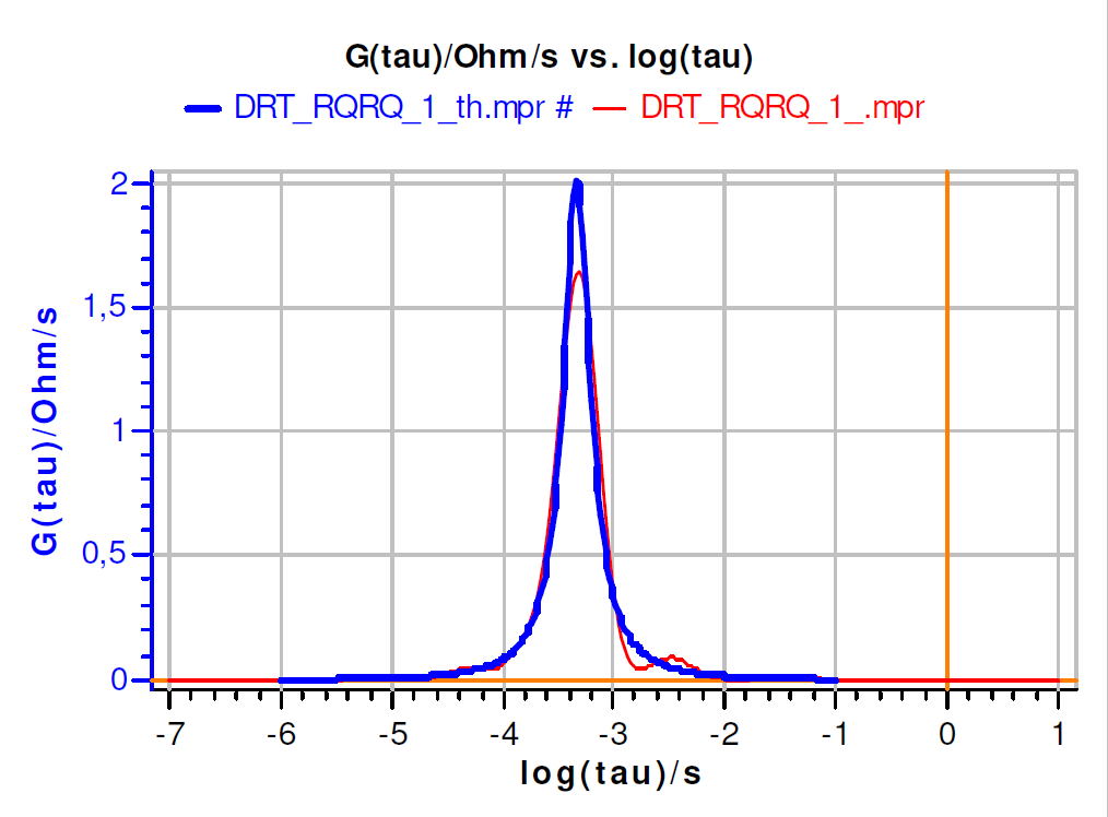
Figure 6 shows the theoretical DRT obtained for the three circuits described in Tab. I. The relationship between G(τ), τ, and the parameters are described by Eq. (3), only in this case it is applied to a sum of R/Q elements.
It is clear that one time constant can be determined on Fig. 6a and two time constants in Figs. 6b and 6c.
The corresponding DRT in Fig. 6a also gives one peak, and hence one time constant.
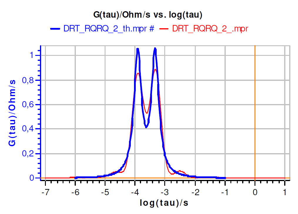
The impedance graph of the second circuit (Fig. 5) is more difficult to interpret as only one time constant can be identified. Even though both R/Qs have different parameters as shown in Tab. I, the corresponding DRT in Fig. 6b shows two peaks, which means two time constants. This would be the main advantage of the DRT representation: it can better resolve the components of a system when two or several time constants are close to one another.
Furthermore, the time constants can be readily accessed by a simple reading on the graph.
Figure 6 also gives the calculated DRT using the DRTtools program and as input the simulated impedance data.
a)
b)
c)
Figure 6: Theoretical (thick blue line) and numerical (thin red line) DRT for a) Circuit 1, b) Circuit 2, c) Circuit 3 in Tab. I.
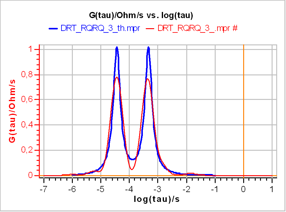
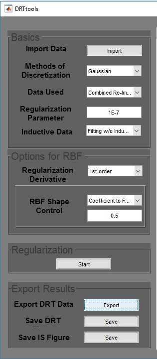
The parameters that were used are shown in Fig. 7. The export tool was used to have data in .txt files and they were imported in EC-Lab® using the “Import file” tool When comparing the theoretical DRT and the DRT obtained by the DRT tools program, one can see that the peak positions are the same and that differences only concern the height of the peak as well the shape. One can notice some oscillations at the bottom of the peaks especially for Figs. 6a and 6b. Differences can be explained by the fact that the numerical solution only approach the analytical solution.

Figure 7: DRTtools interface window showing the parameters used to produce data shown in Fig. 5. Here the data from the second circuit are shown.
Limitations
DRT analysis fit impedance data using an infinite Voigt circuit, whose impedance modulus limits at high and low frequencies do not tend to infinity.
As a consequence, DRT has been used mainly in the field of fuel cells to identify the reaction mechanisms [11,12]. Impedance graphs for such materials have suitable impedance limits at low frequencies.
The method was also used with battery materials [13], which exhibit an increasing impedance modulus at low frequencies. In this case, the DRT analysis is not suitable and the data must be preprocessed to remove the low frequency part i.e the diffusion part of the impedance. Preprocess means that a certain knowledge of impedance analysis is required to be able to use the DRT analysis, whose primary advantage was that it would require no prior knowledge of impedance equivalent circuit analysis.
Additionally, and similarly, an inductive behavior at high frequencies (with an increasing impedance modulus at higher frequencies) is not suitable for DRT analysis.
If impedance data happen to contain an inductive term, several strategies are possible: one can choose to discard the corresponding data with positive imaginary part [14] or, as proposed by DRTtools [10] to account for them in the DRT calculation by adding an inductance term in Eq. (3).
Conclusion
The main advantage of the DRT analysis is that it allows impedance data to be displayed as a distribution of time constants, which can be easier to interpret, can be performed without knowledge of a suitable equivalent circuit and can also reveal time constants not visible on the impedance graph, especially when they are quite close to one another.
The main limitation is that analysis is restrained to impedance graphs for which the limits of the impedance modulus tend to zero both at high and low frequencies.
If this is not the case, preprocessing of the data is needed, which does require knowledge of impedance fitting and analysis and typical shape of equivalent circuits.
Data files can be found in:
C:\Users\xxx\Documents\EC-Lab\Data\Samples\EIS\AN60_X
References
1) P. Agarwal, M. E. Orazem, Luis H. Garcia-Rubio, J. Electrochem. Soc., 139, 7 (1992) 1917.
2) T. H. Wan, M. Saccoccio, C. Chen, F. Ciucci, Electrochim. Acta, 184 (2015) 483.
3) A. Leonide, Ph. D. Thesis, KIT Publishing (2010).
4) A. Leonide, V. Sonn, A. Weber, and E. Iver-Tiff´ee, J. Electrochem. Soc., 155, 1 (2008) 36.
5) T. J. VanderNoot, J. Electroanal. Chem., 386, 12 (1995) 57.
6) F. Ciucci and C. Chen, Electrochim. Acta,
167 (2015) 439.
7) M. Saccoccio, T. H. Wan, C. Chen, and F. Ciucci. Electrochim. Acta, 147 (2014) 470.
8) J. Macutkevic, J. Banys, and A. Matulis, Nonlinear Analysis, Modelling and Control, 9 (2004) 75.
9) J. Weese. Comp. Phys. Com., 111 (1992) 69.
11) H. Schichlein, A. C. Müller, M. Voigths, A. Krügel, and E. Ivers-Tiff´ee, J. Applied Electro-chem., 32 (2002) 875.
12) C. M. Rangel V. V. Lopes and A. Q. Novais. IV Iberian Symposium on Hydrogen, Fuel Cells and Advanced Batteries, Estoril, Portugal, (2013).
13) J. Illig, M. Ender, T. Chrobak, J. P. Schmidt, D. Klotz, and E. Ivers-Tiff´ee, J. Electrochem. Soc., 159, 7 (2012) A952.
14) J. P. Schmidt, E. Ivers-Tiff´ee, J. Power Sources, 315 (2016) 316.
Revised in 08/2019


