

What is CV? A comprehensive guide to Cyclic Voltammetry
Latest updated: April 29, 2026Cyclic Voltammetry: A key electrochemistry technique
Cyclic Voltammetry is, along with EIS (Electrochemical Impedance Spectroscopy), one of the key techniques used to study the kinetics of electrochemical reactions.
Cyclic Voltammetry extends from the more basic step methods such as chronoamperometry and potentiometry. Voltammetry is, in fact, a contraction of voltamperometry, meaning that the current is measured as a function of the voltage (or potential).
With the step methods, one needs to measure the long-time or (steady-state) response of a system to a series of potential or current steps in order to access its complete electrochemical behavior, namely its $I\,vs.E$ characteristic. In terms of execution, this can be quite time-consuming, and the resulting $I\,vs.E$ curve could itself be difficult to analyze.

These two pitfalls can be overcome by recording the current response to a potential sweep $\text{d}E/\text{d}t$ or $v_{\text{b}}$, directly producing the $I\,vs.E$ characteristic.
This potential sweep, most commonly a linear ramp (but it could be a sine wave…), is generally performed at rates ranging from 10 mV/s to 1 V/s for conventional, millimetric electrodes. With smaller micrometric or submicrometric electrodes, sweep rates can reach up to 1 MV/s.
The current is recorded as a function of the potential, which is equivalent to recording versus time. One needs to define two limits between which the potential is scanned. In this case, the technique is simply called Linear Scan Voltammetry (LSV) (Figure 1a). If between these two potentials, we want the voltage to be repeatedly swept between two vertex potentials, the technique is then called Cyclic Voltammetry (CV) (Figure 1b).
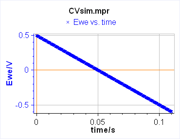
a)
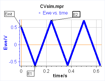
b)
Figure 1: Schematic description from EC-Lab of a) Linear Scan Voltammetry and b) Cyclic Voltammetry.
In both cases, the current is recorded, and the main output is an $I\,vs.E$ curve.
In this topic, we will try to cover a broad range of technical aspects concerning Cyclic Voltammetry. First of all, we will introduce the notions of reversibility, and then describe how Cyclic Voltammetry can be used and which useful information can be obtained, introducing two important tools in EC-Lab®: CV Sim and CV Fit.
We will then discuss the specific subject of steady-state voltammetry, and more precisely, which factors allow it to be carried out.
Thirdly and finally, we will move on to experimental and instrumental considerations and provide guidelines to optimize the setup as well as the experimental settings of voltammetric measurements.
What information can I obtain with Cyclic Voltammetry?
In this section, we will present how Cyclic Voltammetry can be used to determine whether the behavior of the reaction is reversible or irreversible, or neither reversible nor irreversible, and which relationships can be used to determine kinetic parameters such as the standard reaction rate constant or the diffusion constant of the electroactive species.
We will focus on the simplest example, the E reaction:
$$\text{A} + n\text{e}^-\overset{K_\text r}{\underset{K_\text o}{\Leftrightarrow}}\text{B}\tag{1}$$
Where $\text{A}$ and $\text{B}$ are the reducing (oxidized) and oxidizing (reduced) species, respectively, $n$ the number of electrons involved in the reaction, $K_\text r$ and $K_{\text{o}}$ the electronic transfer rate constants of the reduction and the oxidation reaction respectively.
CV Sim and CV Fit allow users to study more complex reactions: EE, EC, CE, EEE and so on…
When the steady-state potential of the electrode $E$ is equal to the standard equilibrium potential of the redox couple $E^{\circ}_\text{A/B}$, then $K_\text r = K_\text o =k^{\circ}$ with $k^{\circ}$ the standard reaction rate constant.
CV Sim and CV Fit
CV Sim (Cyclic Voltammetry simulation) and CV Fit (Cyclic Voltammetry Fitting) are tools dedicated to the Cyclic Voltammetry technique, in the same way, that Z Sim and Z Fit are dedicated to Electrochemical Impedance Spectroscopy. These tools are available in EC-Lab®, BioLogic’s control, and analysis software. These tools, which are excellent for teaching, are available in a demo version of EC-Lab®.
CV Sim and CV Fit can be accessed using the following path in EC-Lab®: Analysis>General Electrochemistry (Figure 2). CV Fit will appear greyed-in because no data are currently opened. Once any $I\,vs.E$ curve is opened or created using CV Sim, the CV Fit tool will become active.

Figure 2: How to access CV Sim and CV Fit in EC-Lab®
The CV Sim window shows two tabs, one is the type of reaction that is being simulated, along with the initial parameters (Figure 3), and the second shows other simulation parameters such as the type of electrode, the voltage limits, the scan rate, other experimental artefacts such as the ohmic drop, measurement noise, double layer capacitance (Figure 4).

Figure 3: CV Sim tab from EC-Lab with the type of reaction,
direction, kinetic parameters and experimental conditions

Figure 4: CV Sim setup tab with electrode shape and radius,
voltage limits, scan rate, and additional artefacts.
Rapid, sluggish, reversible, or irreversible reaction?
When studying the kinetics of an electrochemical (or chemical) process, one important piece of information the user should know is whether the behavior of the electrochemical reaction of interest is reversible, irreversible, or neither reversible nor irreversible (also referred to by Faulkner and Bard as quasi-reversible [1, p. 104]). The reversible behavior of a reaction will lead to different solutions and expressions when trying to analytically solve the kinetic equations.
The value of the reaction rate constant $k^{\circ}$ defines whether the heterogeneous electronic transfer reaction is rapid or sluggish [1, p. 96]. A rule of thumb is that $k^{\circ}\,\geq\,1\,\text{cm s}^{-1}$ is considered large, and the corresponding reaction fast or rapid. If $k^{\circ}\,\leq \,10^{-5}\,\text{cm s}^{-1}$, it is considered small and the reaction slow or sluggish.
Reversibility is somewhat more complex as it depends on various parameters, and one of them only is the value of $k^{\circ}$. The behavior of a reaction is said to be kinetically reversible when the full reaction rate $v(t)$ is small with respect to the partial oxidation or reduction rates, $v_{\text{o}}(t)$ and $v_{\text{r}}(t)$, respectively [2, p. 135]:
$$v_\text o (t)\gg v(t) \, \text{and}\, v_{\text{r}}(t) \gg v(t)\Leftrightarrow v_\text o(t)\approx v_{\text{r}}(t) \tag{2}$$
The corresponding redox system is called Nernstian.
The reaction is said to be irreversible when one of the partial reaction rates is much larger than the other one and, consequently, the full reaction rate is almost equal to the larger partial reaction rate.
In other terms, in the oxidation direction:
$$ v_{\text{r}}(t)<< v_{\text{o}}(t) \iff v(t)\approx v_{\text{o}}(t) \iff v_{\text{r}}(t)<< v(t) \tag{3}$$
and in the reduction direction:
$$v_{\text{o}}(t)<< v_{\text{r}}(t) \iff v(t)\approx v_{\text{r}}(t) \iff v_{\text{o}}(t)<< v(t) \tag{4}$$
It is a mistake to consider that a large $k^{\circ}$ only, corresponds to a reversible behavior as the reaction rate $v(t)$ depends both on the electronic transfer and the interfacial concentrations of the electroactive species, themselves governed by mass transport laws and the potential scan rate.
The determination of kinetic factors
Using CV Sim, we can demonstrate that by performing Cyclic Voltammetries at various scan rates and recording the peak and the current potentials, one can determine whether the behavior of the considered reaction is reversible, irreversible, or neither reversible nor irreversible. Other kinetic factors can also be accessed, once the reversible behavior of the reaction is determined.
Reversible reaction
Let’s open CV Sim, and simulate a few $I\,vs.E$ curves.
Let us consider an E reaction in the reduction direction with $z=1$, $E^{\circ}=0.2\, V$, $\alpha_{\text{f}}=0.5$, $k^{\circ}=10\,\text{cm s}^{-1}$, $C_{\text{A}}=10^{-5}\,\text{mol cm}^{-3}= 10^{-2}\,\text{mol L}^{-1}$, $C_{\text{B}}=0$, $D_{\text{A}}=D_{\text{B}}=10^{-6}\,\text{cm}^{-2}\,\text{s}^{-1}$.
$k^{\circ}$ was chosen so that the reaction can be considered rapid, favoring a priori, a reversible behavior.
In the Setup tab, let us enter the following parameters: Geometry = Linear semi-infinite, Radius $=1$ mm, 800 points per scan, no ohmic drop or double layer capacitance, $E_{\text{init}}=E_1=0.5\,\text{V},\,E_2=-0.3\,\text{V}$.
The scan rates $v_{\text{b}}$ will be chosen according to the following relationship:
$$v_{\text{b}_{n+1}}=4 v_{\text{b}_n}\tag{5}$$
with $n$ an integer and $v_{\text{b}_0}\,=\,10\,\text{V s}^{\text{-1}}$.
The results are shown in Figure 5 for $n+1\,=\,5$. Both the peak potential and current, $E_{\text{p}}$ and $I_{\text{p}}$, are noted.
We can see that $E_{\text{p}}$ is constant while $I_{\text{p}}$ increases (in absolute value), which demonstrates that the redox system is a Nernstian system or the reaction has a reversible behavior.
The expression of the peak current $I_{\text{p}}$ is then given by:
$$ I_{\text{p}}\,=\,-0.446AzF C_{\text{A}}\sqrt{zf_\text N v_{\text{b}}D_{\text{A}}}\;;f_\text N\,=\,F/RT\tag{6}$$
where $A$ is the surface of the disk electrode, $R$ is the perfect gas constant, $F$ is the Faraday constant and $T$ is the temperature.

Figure 5: $I\,vs.E$ curves with increasing scan rates
and $k^{\circ}\,=\,10\,\text{cm s}^{-1}$.
Equation 6 can be used to calculate the diffusion coefficient of the electroactive species A.
It should be noted that the 0.446 coefficient in Eq. 6 only holds for a reversible reaction or (Nernstian system), in our case the lower scan rates of Fig. 5. For example, at 2560 V/S, this coefficient is not 0.446, but 0.444. 0.446 is the theoretical value given by Faulkner and Bard [1, p. 231]. This means that if we scan the potential fast enough, we can slightly shift from a reversible to an irreversible reaction.
Furthermore, Eq. 6 and the factor 0.446 only hold if species B is initially absent from the solution. If this is not the case in your experiment, you can use CV Sim to calculate the right value of the factor and then use this value to recalculate the diffusion coefficient. This is better explained in the corresponding Learning Center article – Using CVSim as a Learning tool with more detailed information in Application Note 41-1.
For YouTube video tutorials on how to obtain and interpret these curves please see the CVSIM videos part 1 and Part 2.1 below
Irreversible reaction
Let’s go back to CV Sim and set $k^{\circ}\,=\,0.001\,\text{cm s}^{-1}$, all the other parameters being the same. With such a small $k^{\circ}$ we can infer that the reaction is sluggish, and its behavior a priori, irreversible.
The different $I\,vs.E$ curves are given in Figure 6. Both $E_{\text{p}}$ and $I_{\text{p}}$ change with the scanning rate, which demonstrates that the reaction is irreversible.
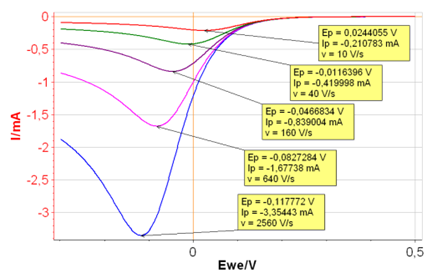
Figure 6: $I\,vs.E$ curves with increasing scan rates
and $k^{\circ}\,=\,0.001\,\text{cm s}^{-1}$.
The equation 6 now becomes:
$$ I_{\text{p}}\,=\,-0.496AzF C_{\text{A}}\sqrt{\alpha_{\text{r}}f_\text N v_\text b D_{\text{A}}}\;;f_\text N \,=\,F/RT\tag{7}$$
With $\alpha_{\text{r}}$ being the symmetry factor of the reaction in the reduction direction. $\alpha_{\text{r}}$ + $\alpha_{\text{o}}$ = 1, with $\alpha_{\text{o}}$ being the symmetry factor of the reaction in the oxidation direction.
Equation 7 can be used to determine $D_{\text{A}}$ or $\alpha_{\text{r}}$ and is given by Bard and Faulkner [1, p. 236].
The peak potential $E_{\text{p}}$ is proportional to $\ln v_\text b$ following this relationship [1, p. 236]:
$$E_{\text{p}}\,=\,E^{\circ}+\frac{1}{\alpha_{\text{r}}nf_\text N}\left(0.78+\ln\frac{k^{\circ}}{\sqrt{\alpha_{\text{r}}nf_\text N v_\text b D_{\text{A}}}}\right)\tag{8}$$
In this case, the standard reaction constant $k^{\circ}$ can be determined as well as the symmetry factor $\alpha_{\text{r}}$.
Again, more detailed information can be found in Application Note 41-1.
For a YouTube video tutorial on how to obtain and interpret these curves please watch CVSIM video part 1 (above) and Part 2.2 (below)
Steady-state voltammetry
Why work in a steady-state?
In this part of this Cyclic Voltammetry article, we will discuss the notion of steady-state. As mentioned earlier, when it was not possible to program a voltage ramp, the only way to plot the $I\,vs.E$ characteristic of a system was to apply a potential or current step and then record the response at long times when it was constant. This way the steady-state $I\,vs.E$ characteristic could be constructed, but with this approach, it would be time-consuming. The electrochemical response of a redox system in steady-state is easier to analytically describe, as any time-dependent term is equal to 0.
This is for example the case for a Rotating Disk Electrode (RDE): the measurement of the steady-state mass-transport-controlled current allows users to easily reach important kinetic parameters such as the diffusion coefficient, symmetry parameter $\alpha$ and the already mentioned standard reaction constant $k^{\circ}$ using Levich and Koutecký-Levich equations. More information can be found in the corresponding article: rotating disk electrode, how does the Koutecký-Levich analysis work?. Furthermore, steady-state is also a requirement in Electrochemical Impedance Spectroscopy (EIS).
How do I know the voltammetric curve was performed in steady-state conditions?
The simplest way to recognize a steady-state voltammetric curve is to see if the forward and backward potential scans give the same current response. In other words, the two parts of the curves are superimposed, as is illustrated in Figs. 7a and c.
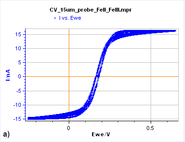
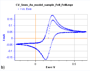
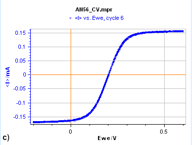
Figure 7: Cyclic Voltammetry curves obtained on a) a 15 µm diameter Au disk b) a 5 mm diameter Au disk, and
c) a Rotating 2 mm Pt Disk Electrode (RDE). (Conditions: 5 mM FeII/FeIII, 0.1 M KCl, potential ranges: 0 V/OCP,
0.650 and -0.250 V/Ag/AgCl a) and b) 10 mV/s, c) 25 mV/s, 5000 rpm).
Figure 7a is the $I\,vs. E$ response obtained on a 15 µm diameter disk electrode (also called an UltraMicroElectrode, UME). When the potential is scanned backward or forward, it produces the same curve (although we can see a slight shift) with a typical S-shape. In this case, what we see is a steady-state curve. If the potential scan is stopped and the potential held at a certain value, the current value remains constant.
Figure 7b shows the same experiment but performed on a 5 mm Au disk electrode. The shape is totally different as the forward and backward scans are not superimposed. In this case, the steady-state conditions are not reached. If the potential scan is stopped and the potential held at a certain value, the current decreases and reaches 0.
Finally, in Figure 7c, the Cyclic Voltammetry measurement was performed on a Rotating Disk Electrode (RDE). In this case, also, it can be seen from the shape of the curve that we are in steady-state conditions. The same S-shaped curve as in Fig. 2a can be seen. Again, as for the UME curve, if the potential scan is stopped and the potential held at a certain value, the current value remains constant.
Also, it can be seen in Figs. 7a and 7c, on steady-state curves that for a given potential range, the current does not change with potential anymore. At these potential ranges, the current depends on mass transport conditions, interfacial concentrations, and diffusion coefficients.
In electrochemistry, steady-state conditions mean that at any point of the curve the species concentrations do not vary over time, only with the distance from the electrode. The overall reaction rate and consequently the current are constant with time.
The influence of the electrode geometry and the mass transport conditions
Now we will explain why steady-state conditions can only be reached with a UME or an RDE but not with large planar electrodes.
We will take a step back here and describe what happens at each electrode interface when we apply a potential step in Cottrell conditions, again examining the E reaction. In Cottrell conditions, a large amplitude potential step is applied to the mass-transport region. The concentration of the electroactive species is zero at the electrode/electrolyte interface and the Faradaic current is controlled by mass transport. Electroactive species are being produced/consumed and their concentrations, in the vicinity of the electrode, change with time, creating concentration gradients.
Figures 8, 9 and 10 show for a given time $t_0$, is concentration lines and diffusion/current fluxes for three types of electrode geometries: a large conventional planar electrode (Fig. 8), a hemispherical electrode (Fig. 9), and a disk Ultra MicroElectrode (UME) (Fig. 10), which we can simply define as a disk electrode with a radius of around 25 µm or lower.
In the case of the large planar and the hemispherical electrodes, the isoconcentration lines are parallel to the electrode surface (blue lines in Figs. 8 and 9). The electroactive species’ mass transport occurs by diffusion, perpendicularly to the isoconcentration lines as indicated by the arrows (yellow arrows in Figs. 8 and 9). For a conventional planar electrode, the diffusion is linear semi-infinite and hemispherical semi-infinite for a hemispherical electrode.
Figure 8: Isoconcentration lines and geometry of diffusion at a conventional planar
electrode at a given time. The blue lines are isoconcentration lines. The concentration
outside of the furthest line from the electrode is the bulk concentration. The orange arrows
show diffusion fluxes of electroactive species and current lines.

Figure 9: Isoconcentration lines and geometry of diffusion at a hemispherical electrode at a given time.
The blue lines are isoconcentration lines. The concentration outside of the furthest line from the electrode
is the bulk concentration. The orange arrows show diffusion fluxes of charged species and current lines.
In the case of a disk UME, it is a bit more complicated as diffusion at a UME is linear semi-infinite, and augmented by a radial component at the edges of the electrode (Fig. 10).
In the case of a Rotating Disk Electrode (RDE), the augmentation of mass-transport is performed by convection, which allows it to behave in a manner similar to a UME and a hemispherical electrode.
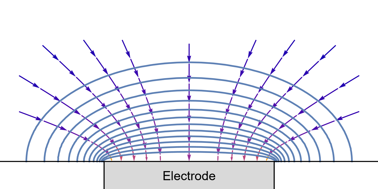
Figure 10: Isoconcentration lines and geometry of diffusion at an Ultra Micro Electrode at intermediate times.
The blue lines are isoconcentration lines. The arrows show diffusion fluxes of charged species and current lines.
The edge effects can be seen: the current and diffusion lines are not always perpendicular to the surface.
Different mass transport conditions mean different boundary conditions and lead to different solutions of the mass transport equations, and eventually current-potential equations. This is described in great detail in the books by Faulkner and Bard [1, Chapter 5] and Diard, Le Gorrec, and Montella (in French) [2, Chapter II].
Let us now examine how the concentrations at the interface and the concentration profile away from the electrode change with time for each geometry.
In the case of a large planar electrode (linear diffusion) (Fig. 11), in Cottrell conditions, the depletion region, ie the region where concentration gradients exist, will grow indefinitely with time and, in the case of voltammetry, with the potential. Eventually, the concentration gradient at the electrode surface and the current will reach zero as can be seen in Fig. 11.

Figure 11: left) $I vs. t$ at the electrode/electrolyte interface, right) $ C\,vs.x$ at times shown in the left figure, in the case of a
large planar electrode where semi-infinite linear diffusion occurs in Cottrell conditions, for the reversible redox reaction
E, $\text{A}\,+\,n\text{e}\,\rightarrow\, \text{B}$. $C$ is the concentration of species $\text{A}$ and $x$ the distance normal
to the planar electrode.
In the case of a hemispherical electrode, a disk UME, or an RDE, depletion will only occur in a definite and constant length, because the diffusion field is able to draw material from a continually larger area at its outer limit. After a certain time, the concentration gradient at the interface and the current are constant with time and with potential, in the case of voltammetry, as can be seen in Fig. 3.

Figure 12: left) $I\,vs. t$ at the electrode | electrolyte interface, right) $ C\,vs.x$ at times shown in the left figure,
in the case of an hemispherical electrode, or a disk UME, or an RDE where semi-infinite linear diffusion, radial
diffusion or diffusion-convection, respectively, occurs in Cottrell conditions, for the reversible redox reaction
E, $\text{A}\,+\,n\text{e}\,\rightarrow\, \text{B}$. $C$ is the concentration of species $\text{A}$ and $x$ the
distance normal to the center of the electrode.
To summarize, steady-state conditions can be reached when the electroactive species depletion/enrichment region which results from the redox reaction has a finite dimension, that does not change with time, and the concentration gradient, at the interface is constant. This is possible only when sufficient electroactive species are available thanks to additional mass transport by convection (RDE), radial (UME), or hemispherical diffusion (hemispheric electrode) compared to linear diffusion at a large planar electrode.
Let us now return to voltammetry and see what happens when we change the potential of the electrode linearly with time.
The influence of the scan rate
The effect of scan rate can be inferred by considering that the larger the scan rate, the smaller the duration of the potential scan and the less likely the steady-state regime will be reached, considering steady-state corresponds to the state of the system at infinite time. This means that even though diffusion conditions are such that steady-state conditions could be reached, if the scan rate is too fast, the $I\,vs.E$ characteristic of the system will not be steady-state.
This is illustrated in Fig. 13, which shows the evolution of $I\,vs.E$ on the left and the interfacial concentrations of electroactive species on the right with the scan rate in the case of a hemispherical electrode of 10 µm radius. These curves were obtained using CV Sim.
At lower scan rates (1 and 10 mV/s), we can see on the left, that the diffusion current plateaus, and both backward and forward scans are superimposed. On the right, we can see that the interfacial concentration of the produced species is maximal. From 100 mV/s to 10 V/s, we can see on the left the curves are not steady-state anymore: the current plateau disappears, the forward and backward scans are not superimposed, and on the right, the interfacial concentration of the produced species is not maximal anymore.
These results could also apply to a UME and an RDE.

Figure 13 : Evolution of left) $I vs. E$ curve and right) interfacial concentrations with scan rate for the
redox E reaction $\text{A}\,+\,n\text{e}\,\rightarrow\, \text{B}.\; \text{Parameters}:n=1,\, E^{\circ} = 0.2\,\text{V},\, k^{\circ} = 0.01\,\text{cm}\,\text{s}^{-1},\, \alpha_\text f = 0.5,\, C^*_\text{A} = 0.01\,\text{mol}\,\text{L}^{-1},\, C^*_\text{B} = 0,\, D_\text{A} = 10^{-5}\,\text{cm}^2\,\text{s}^{-1},\, D_\text{B} = 5\times10^{-6} \,\text{cm}^2\,\text{s}^{-1},\, r_0 = 10\,$µ$\text{m}$.
Let us now compare the $I\,vs.E$ obtained on a large planar electrode and at a hemispherical electrode of the same size at different scan rates. Figure 14 shows the $I\,vs. E$ curves for linear (in blue) and spherical (in red) diffusion at different scan rates. We can see that the faster the scan rate, the more similar both curves are. As the scan rate gets lower, the red curve corresponding to a hemispherical electrode tends to be a typical steady-state curve, with superimposed backward and forward scan and current plateaus. As the scan rate increases, the behavior of a hemispherical electrode and a planar electrode of the same size are the same.
The same behavior as the hemispherical electrode could be seen for a UME or an RDE. The curves in Fig. 14 were obtained with CV Sim.

Figure 14: Comparison of the $I\,vs.E$ curve for a linear semi-infinite diffusion (blue curve)and spherical semi-infinite diffusion (red curve) for various scan rates. $\text{A}\,+\,n\text{e}\,\rightarrow\, \text{B}.\; \text{Parameters}: n=1,\,E^{\circ} = 0.2\,\text{V},\, k^{\circ} = 0.01\,\text{cm}\,\text{s}^{-1},\, \alpha_f = 0.5,\, C^*_\text{A} = 0.01\,\text{mol}\,\text{L}^{-1},\, C^*_\text{B} = 0,\, D_\text{A} = 10^{-5}\,\text{cm}^2\,\text{s}^{-1},\, D_\text{B} = 5\times10^{-6} \,\text{cm}^2\,\text{s}^{-1},\, r_0 = 1\,\text{mm (linear diffusion)},\, r_0 = 0.707\,\text{mm (spherical diffusion)}$
To summarize, we can say that:
- It is not possible to perform steady-state voltammetry on a large (millimetric) quiescent planar electrode.
- In systems where steady-state voltammetry is possible, according to diffusion conditions (hemispherical electrode, UME, RDE), there always exists a scan rate value high enough so that diffusion conditions become linear, and conditions are not steady-state anymore, as is the case on a large planar electrode.
These two experimental sets of conditions, the diffusion mode and the scan rate, can be contained within one single parameter that is called the sphericity parameter, which we describe in the next part of this topic.
The sphericity parameter
The sphericity parameter $L$ is a dimensionless parameter defined as follows for a redox reaction $\text{A}\,+\,n\text{e}\,\rightarrow\, \text{B}$ occurring on an electrode with a radius $ r_{\text{hemi}}$.
$$L= r_{\text{hemi}}\sqrt{\frac{|n|f_\text{N}v_{\text{b}}}{D_\text{O}}}\tag{9}$$
With $n$ the number of exchanged electrons, $f_\text{N}=F/(RT)$, $v_{\text{b}}$ the scan rate and $ D_\text{O}$ the diffusion coefficient of the electroactive species $\text{O}$.
In case you are using a planar electrode, you can also use the equation above by assuming that $r_{\text{hemi}}=0.07 r_{\text{disk}}$ where $r_{\text{disk}}$ is the radius of a disk electrode [3]. It shows that there is an equivalence between hemispherical and linear+radial diffusion.
When $L \rightarrow +\infty$ then we are in the case of a linear semi-infinite diffusion and hence no steady-state voltammetry is possible. It is easy to see that the condition $L \rightarrow +\infty$ corresponds to a large $r$ so a large electrode, or large $v_\text b$ ie fast scan rates.
On the opposite, when $L \rightarrow 0$, we are in the conditions of a hemispherical diffusion, which means that steady-state or quasi steady-state voltammetry can be performed. The curve then shows a plateau at the limiting current $i_\text{lim} = 2\pi FD_\text{O}C_\text{O}^*r$. The condition $L \rightarrow0$ corresponds to either a small $r$ so a small electrode, or small $v_\text b$ ie slow scan rates.
One could add that the sphericity parameter could be better-named as a “linearity parameter”, as the magnitude of $L$ quantifies the degree of linearity of diffusion in the case of a hemispherical (or a UME) electrode.
Figure 15 shows the evolution of $I\,vs. E$ curves in the case of a hemispherical diffusion. We can see that we move from a steady-state curve to a quasi-steady-state curve to a non-steady-state curve, like the linear diffusion case. The only parameter that changes is the radius of the electrode that is changing from 0.01 mm in the case of the steady-state curve to 0.1, 1, and finally 10 mm. The evolution of the corresponding $L$ parameter is shown in the graph.

Figure 15: $I\,vs. E$ curves for a spherical semi-infinite diffusion for $r$ varying from 0.01 to 10 mm by decades. $E^\circ$ = 0.2 V; $k^\circ$ = 0.01 cm s-1 ; $\alpha_f$ = 0.5 ; $C^*_\text{A}$ = 0.01 mol L-1 ; $C^*_\text{B}$ = 0 ; $D_\text{A} = 10^{-5}$ cm² s-1 ; $D_\text{B} = 5\,\times\,10^{-6}$ cm² s-1. The evolution of the $L$ parameter in these conditions is shown.
The same type of graphs can be obtained for a fixed radius by increasing the scan rate. This is shown in Fig. 16, which we plot again here below but instead of the scan rate, we plot the $L$ parameter, which characterizes only the “spherical” diffusion ie the red curve below.

Figure 16: Comparison of the $I\,vs. E$ curve for a linear semi-infinite diffusion (blue curve) and spherical semi-infinite diffusion (red curve) for various scan rates from 0.01 to 100 mV/s per decade. $E^\circ$ = 0.2 V; $k^\circ $ = 0.01 cm s-1 ; $\alpha_f$ = 0.5 ; $C^*_\text{A}$ = 0.01 mol L-1 ; $C^*_\text{B}$ = 0 ; $D_\text{A} = 10^{-5}$ cm² s-1 ; $D_\text{B} = 5\,\times\,10^{-6}$ cm² s-1 ; $r_0$ = 1 mm (linear diffusion) ; $r_0$ = 0.707 mm (spherical diffusion). The $L$ parameter is shown for the spherical diffusion (red curve).
It can be seen in Fig. 16, that the discrepancy between the linear and spherical behavior occurs below a value of L = 62.4 and above a value of 19.7, for the set of parameters described in Figure 16 caption.
We can more precisely evaluate when this discrepancy occurs by plotting the ratio $I_{\text{p, lin}}/ I_{\text{p, sph}} \,vs. \,L$ where $I_{\text{p, lin}}$ and $I_{\text{p, sph}}$ are the forward peak currents for the linear and the spherical diffusion, respectively. This is shown in Fig. 17. The plotted point corresponds to a ratio of 95% and an $L$ value of ≈ 32. This number only holds for the set of parameters shown in Fig. 16. Above this value, diffusion occurs linearly (even if the electrode is hemispherical). Below this value, edge effects (radial diffusion) start to appear.
Figure 18 shows the combination of $r$ and $v_{\text{b}}$ for which $L\,=\,32$, that defines the boundary between linear diffusion and linear diffusion with radial components, for a hemispherical electrode in the conditions given in the Fig. 16 caption.

Figure 17: Evolution of the ratio $I_{\text{p, lin}}/ I_{\text{p, sph}} \,vs. \,L$ $(10^{1.5}=32)$.
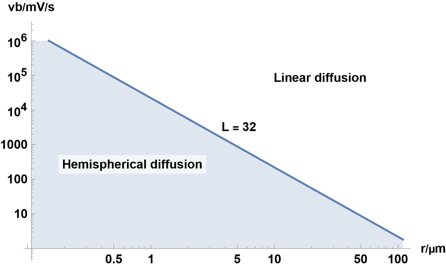
Figure 18: $v_{\text{b}}\,vs.r$ with $L\,=\,32$, where $r$ is the radius of the hemispherical electrode.
Any $v_{\text{b}}$ and $r$ combination which falls in the light blue area corresponds to conditions where
spherical diffusion starts to occur, for parameters described in the Fig. 16 caption.
To summarize, we can say that the sphericity (or linearity) factor defines, in the case of a simple E reaction with only reacting species A in the solution, the scan rate and the electrode size combinations for which linear diffusion can occur, preventing steady-state conditions from being reached, even in the case of a UME or a hemispherical electrode. CV Sim can be used to perform the same study on a different set of parameters.
Instrumental and experimental considerations
In the last part of this topic, we will discuss various instrumental and experimental factors to account for when performing Cyclic Voltammetry measurements:
- What to do when the ohmic drop and double-layer capacitance are non-negligible?
- How do I set up the parameters of the CV technique?
- What is an Analog Ramp Generator and when do I need it?
The effect of the ohmic drop and the double layer capacitance
Double-layer capacitance
The electrode | electrolyte interface, which is a metal-solution junction, behaves, as a first approximation, like a capacitor. When polarizing an electrode in an electrolyte where electroactive species can be reduced or oxidized at the interface, the current is the sum of a Faradaic current $I_{\text{f}}$, related to the redox reaction, and a capacitive current $I_{\text{c}}$ related to the electrical charge transfer due to the double layer capacitance.
$$I=I_{\text{c}} + I_{\text{f}}\tag{10}$$
The capacitive current depends on time-derivative of the potential $E(t)$ and the double layer capacitance $C_{\text{dl}}$:
$$ I_{\text{c}}=C_{\text{dl}}\left(\frac{\text{d}E}{\text{d}t}\right) \tag{11}$$
In the specific case of a voltage sweep at a scan rate $v_{\text{b}}$, $\text{d}E/\text{d}t=v_{\text{b}}$ and
$$ I_{\text{c}}=C_{\text{dl}} v_{\text{b}}\tag{12}$$
The ohmic drop
In a three-electrode cell configuration, the ohmic drop is the resistance between the working electrode and the reference electrode. This resistance $R_\Omega$, modifies the potential « seen » by the electrode $V(t)$ compared to the potential value applied by the potentiostat $E(t)$ by a value $R_\Omega I(t)$ with $I\lt0$ for a reduction current and $I\gt0$ for an oxidation current (Figure 19):
$$V(t)=E(t)+R_\Omega I(t) \tag{12}$$
If we move on to the special case of Cyclic Voltammetry, with $v_{\text{b}}$ the scan rate and $E_{\text{init}}$ the initial potential, we have:
$$E(t)= E_{\text{init}}+ v_{\text{b}}(t)- R_\Omega I(t) \tag{13}$$

Figure 19: A three-electrode setup with the illustration of the ohmic drop and the double-layer capacitance.
How does this affect measurements?
Using CV Sim the effects of both non-negligible ohmic drop and double layer capacitance can be simulated.
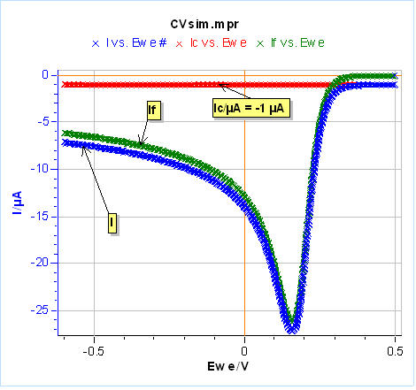
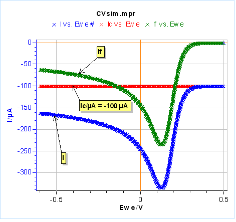
Let’s use the same parameters as in Fig. 3 and 4, except for $C_{\text{dl}}$ that we set at 100 µF and we use an electrode radius of 1 mm. We performed one half-cycle for the sake of simplicity. The results are shown in Figure 20a. The capacitive current in red leads to a negative shift of the total current in blue compared to the Faradaic current in green. In Figure 20a, the capacitive current could be considered negligible because we are scanning relatively slowly. It can be a problem at higher scan rates for example at 1 V/s where the capacitive current is around one-half of the Faradaic current (Fig. 20b). One can see that the capacitive current can be determined when the voltage scan starts and the total current is equal to the capacitive current.
By way of a reminder, it is important to note that the capacitive current is proportional to $v_\text b$, whereas the Faradaic current is proportional to $\sqrt{ v_\text b}$ (Eqs. 6 and 7). It must be noted that for very high scan rates, the capacitive current might overshadow the Faradaic current.
a)
b)
Figure 20: Total, Faradaic and capacitive currents in blue, green and red, respectively, $vs.E$ simulated using CV Sim and the conditions shown in Fig. 3 and 4 with a radius of 1 mm and a $C_{\text{dl}}$ value of 100 µF. a) $v_{\text{b}}=10\,\text{mV}\text{s}^{\text{-1}}$, b) $v_{\text{b}}=1\,\text{V}\text{s}^{\text{-1}}$
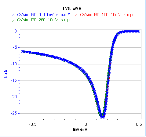
Let us now set $C_{\text{dl}}=0$ and $ R_\Omega=20\,\Omega$, the results are given in Figure 21 for the same scan rates as in Fig. 20. It can be seen that at low scan rates, in our case 10 mV/s, the ohmic drop has little influence on the Faradaic current (Fig. 21a). Its influence can be seen at higher scan rates, which means larger currents (Fig. 21b). Unlike capacitance, both the peak current and potential are shifted: the peak current is larger in absolute value and the peak potential is shifted to more negative values for a reduction reaction (more positive values for an oxidation reaction).
a)

b)
Figure 21: Total current with different ohmic drop values, simulated using CV Sim and the conditions shown in Fig. 3 and 4 with a radius of 1 mm.
a) $v_{\text{b}}=10\,\text{mV}\,\text{s}^{\text{-1}}$, b) $v_{\text{b}}=1\,\text{V}\,\text{s}^{\text{-1}}$
For more detailed information and a description of the combined effects of both non-negligible ohmic drop and double layer capacitance, please read the Application Note 41-2 CV Sim: Simulation of the simple redox reaction (E) Part II: The effect of ohmic drop and double layer capacitance.
For the various methods available to compensate for ohmic drop please take a look at the following Learning Center article (ohmic drop correction, a means of improving measurement accuracy with potentiostats and the corresponding application notes.
The numeric ramp
When we add a Cyclic Voltammetry technique, there are quite a number of settings as shown in Fig. 22. The parameters “Ei”, “E1”, “E2” have already been explained at the beginning of the article. The scan rate $v_{\text{b}}=\text{d}E/\text{d}t$ was also explained before, but because we are using an instrument that is numerically controlled, the voltage ramp is not exactly linear but rather a succession of small voltage steps (Fig. 23). $\text{d}E$ is defined by the potential range $\text{E}_{\text{range}}$ and the resolution of the Digital-To-Analog (DAC) converter. In the case of BioLogic systems, it is 16 bytes. We then have, assuming a constant $\text{d}E$:
$$\text{d}E=\frac{\text{E}_{\text{range}}}{2^{16}}\tag{14}$$
Then the scan rate $\text{d}E/\text{d}t$ sets the value of $\text{d}t$ and $N$ the number of potential steps over which the average current is recorded, represented by the black dots in Fig. 23. There is one point for each $\text{d}E_{\text{N}} = \text{d}E\,N$. For each step, the current is measured over a certain duration defined as a remaining percentage of $\text{d}t$.
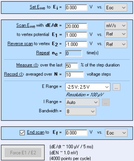
Figure 22: Cyclic Voltammetry settings window.
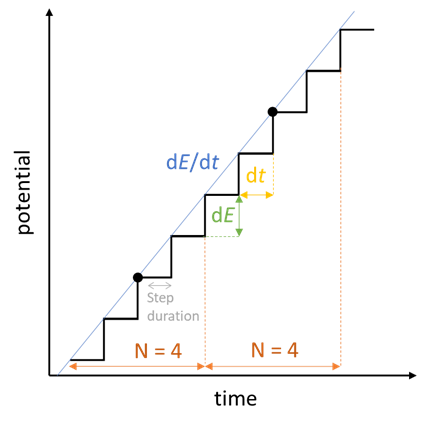
Figure 23: How a voltage sweep is actually performed with the EC-Lab®
CV technique, here in the scan of a positive potential ramp.
The number of data points $N_{\text{data}}$ per cycle is then defined as:
$$N_{\text{data}}=2\frac{\left\lvert E_2-E_1\right\rvert}{\text{d}E_{\text{N}}}\tag{14}$$
With $E_2$ and $E_1$ the vertices potentials. The factor 2 is due to the fact that one cycle is defined as the return to an initial condition: $E_1 \to E_2 \to E_1$.
The benefit of being able to choose the duration the current is recorded at, is that the capacitive contribution of the current can be removed, as it occurs mostly at the beginning of the step. Nonetheless, it is always better to record all contributions and hence set 100%.
The main limitation of the numeric ramp is actually related to the minimum available acquisition time, namely 200 µs, which does not allow the sweeping of potentials at very high rates, because the number of data points is then too low. The following formula can be used to calculate the number of data points for a given scan rate $ v_{\text{b}}$ and time step $\text{d}t$.
$$ N_{\text{data}}=2\frac{\left\lvert E_2-E_1\right\rvert}{v_{\text{b}}\,\text{d}t\,{N}}\tag{15}$$
Scanning from -1 to 1 V, at 100 V/s and averaging over 5 voltage steps gives a number of 40 points per cycle which is rather small. Also, the software ohmic drop compensation requires 400 µs, and it can also be a problem at very high scan rates. In such cases, the Analog Ramp Generator (ARG) option is required.
The Analog Ramp Generator (ARG)
The ARG is an optional board, that can be extremely easily mounted on the channel board, which allows the acquisition time to go down to 1 µs, and hence allows very high scan rates to be used. Furthermore, the capacitive current is also reduced because the shape of the potential ramp is an actual linear ramp and not a succession of steps. At the beginning of each step the potential variation $\text{d}E/\text{d}t$ is very large (almost infinite…) and so the capacitive current is also very large (Eq. 12). This is avoided when using a linear ramp and the capacitive current is constant with time, similarly to the simulation results shown in Fig. 20.
Figure 24 illustrates the effect of using a numerical ramp on the total measured current and how it compares with an analog linear ramp. When the scan rate is very large or for highly capacitive systems, at each potential step there is a huge decrease (or increase for an increasing potential sweep) of the capacitive current, which can lead to a change in the current range, hence decreasing the quality of the current measurement.

Figure 24: Illustration of the effect of highly capacitive systems or very fast scan
rates on the total current when using a numerical ramp or an analog ramp.
Another advantage of the ARG is that it allows the ohmic drop compensation to be performed analogically and not by software, as is generally the case. The software ohmic drop compensation requires a minimum time of 400 µs to be performed, so when using very fast scan rates it cannot be used. With the ARG, the ohmic drop compensation is performed analogically with no specific speed limitation.
Cyclic Voltammetry: A glossary of terms
| Term | Cyclic Voltammetry Definition |
| Analog Ramp Generator (ARG) | Optional device that allows the application of a linear analog voltage ramp to the working electrode instead of a numeric ramp. It is necessary for very fast scan rates and/or studies on highly capacitive systems. |
| Capacitive current | Current related to the charging and discharging of the capacitance created by the electrode/electrolyte interface. |
| Cottrell conditions | Cottrell conditions are reached when the applied potential step leads to an interfacial concentration of the electroactive species of 0. The Faradaic current is then solely dependent on the slope of the concentration profile at the interface. |
| CV Fit | Analysis software available in EC-Lab® that can be used to fit Cyclic Voltammetry data and retrieve kinetic parameters. |
| CV Sim | Companion software of CV Fit available in EC-Lab® that simulates current responses for a large range of redox reactions, electrode geometries, and input potential modulations. |
| Diffusion-convection (Bounded diffusion) | Mass transport conditions where the electroactive species are transported to the electrode by diffusion and convection. The concentration gradient of the reactive species occurs at a finite distance from the electrode and steady-state conditions can be fulfilled. It is generally achieved using a Rotating Disk Electrode (RDE). |
| Disk macro-electrode | Disk electrode, whose size only allows semi-infinite linear diffusion as a mass transport process. Steady-state conditions cannot be fulfilled at this electrode even when scanning at very low scan rates. |
| E reaction | Redox reaction with one single step. A + ne ↔ B |
| EC reaction | Reaction involving two steps and three species: one with electron transfer and another one without electron transfer, just a chemical change of the species. A + ne ↔ B ↔ C |
| EE reaction | Reaction involving two steps and three species, both steps are redox reactions with electron transfers. A + n1e ↔ B + n2e ↔ C |
| Faradaic current | Current related to the electrochemical reaction occurring at the electrode | electrolyte interface. |
| Forward/backward | Forward means in the direction of the desired reaction and backward in the opposite direction. If a reduction reaction is studied, “forward” means the reduction direction; for the potential scan, “forward” means scanning to more negative values. If the oxidation reaction is studied, it is all reversed. |
| Hemispherical diffusion | Diffusion of electroactive species to/from a hemispherical electrode. In these conditions, steady-state conditions can be reached until a certain scan rate. |
| Hemispherical electrode | An electrode that is the half of a sphere and where electroactive species diffuse hemispherically, which allows steady-state conditions to be fulfilled, again until a certain scan rate. |
| Linear diffusion | Mass-transport conditions where electroactive species are transported to the electrode in one direction. It generally occurs on a large disk electrode or any electrode at very high scan rates. Steady-state conditions are not fulfilled. |
| Linear Scan Voltammetry (LSV) | Linear Scan Voltammetry consists of scanning the potential and measuring the current but only to more positive or more negative values. It is one-half of Cyclic Voltammetry. |
| Nernstian reaction behavior | Another name for a reversible reaction behavior. |
| Peak current | When performing CV in non-steady-state conditions, the interfacial depletion of the electroactive species and the decrease of the slope of the concentration profile creates a current decrease (in absolute value) forming a peak. The value of the peak current mainly depends on the scan rate and the diffusion coefficient of the electroactive species. Two different relationships exist whether the reaction is reversible or not. See the following topic for a clearer explanation: https://biologic.net/topics/cvsim-as-a-learning-tool-ii-interfacial-concentrations/ |
| Peak potential | The peak in the I vs. E curve can be used to define a peak potential. For an E reaction, if the peak potential depends on the scan rate, it means that the reaction is irreversible. |
| Radial diffusion | Diffusion of electroactive species to/from the edges of a disk UME. The diffusion fluxes then have two components, unlike in linear diffusion conditions. Steady-state conditions can be reached in this case, until a certain scan rate. |
| Reaction rate | In the case of a redox reaction, the reaction rate defines the Faradaic current. It is equal to the rate of the reaction in the forward direction minus the reaction rate in the backward direction. |
| Reaction rate constant | Constants related to the reaction rate: usually symbolized by the letter k. For a given redox reaction E, the forward, backward, and standard reaction rate constants are defined. The reaction rate standard constant k° defines whether the reaction rate is sluggish (k° ≤ 10-5 cm s-1) or rapid (k° ≥ 10-1 cm s-1). Between these two magnitudes, the reaction can be considered neither rapid nor sluggish… |
| Reversibility | Reversibility or irreversibility is related to the partial reaction rates and how they compare with the overall reaction rate. If the forward and backward reaction rates are equivalent, then the reaction behavior is reversible or Nernstian. If one of the two partial reaction rates is much larger than the other one then the reaction behavior is irreversible. The reversibility or irreversibility of a reaction can be assessed by measuring the potential and current peaks at various scan rates. A reaction can also be neither reversible nor irreversible… The reversibility of a reaction depends on its intrinsic kinetic parameters but also on the condition of the experiments (scan rate, rotation at an RDE). |
| Rotating disk electrode (RDE) | An electromechanical device where a disk electrode is rotated at an accurate speed in a solution containing electroactive species. The controlled mass transport of the electroactive species, by diffusion and convection, allows users to perform steady-state voltammetry and to use analytical expressions (Levich and Koutecký-Levich) to derive kinetic parameters. |
| Scan or sweep rate | The rate at which the potential is scanned during an LSV or a CV. It can affect the reversibility of the reaction behavior and the steady-state conditions. For an electrode of a given size where steady-state conditions can be established (RDE, UME, hemispherical electrode…), the higher the scan rate, the further away we will move from the steady-state conditions. For a given reversible reaction, there is always a scan rate for which the reaction will become irreversible. |
| Semi-infinite diffusion | Diffusion conditions in which the concentration gradient of the electroactive species occurs at an infinite distance from the electrode. Steady-state conditions can be reached only if diffusion occurs hemispherically or radially. |
| Sphericity parameter | It is a theoretical dimensionless parameter that defines, for a given diffusion coefficient, the scan rate and electrode size values for which diffusion occurs linearly, hemispherically, or linearly and radially. This parameter can be used for hemispherical electrodes but also for planar disk electrodes. |
| Steady-state conditions | Conditions for which all the time-dependent parameters are constant. It can be somehow predicted by considering that it is a behavior of a system when time tends to +∞, or very long times. In voltammetry, steady-state conditions mean that at any given point of the I vs. E curve, the current will remain constant if the potential scan was stopped and maintained constant. |
| Ultra Micro Electrode (UME) | Electrode, most commonly a disk, whose size allows mass transport by linear and radial diffusion, similar to hemispherical diffusion. Steady-state conditions can be fulfilled at this electrode until a certain scan rate. |
| Vertex, vertices | Potential value or values between which the potential is scanned during LSV or CV and the scan rate sign is reversed. |
References
[1] A. J. Bard, L. R. Faulkner, Electrochemical Methods: Fundamentals and Applications, Wiley, Hoboken, (2001).
[2] J.-P. Diard, B. Le Gorrec, C. Montella, Cinétique Electrochimique, Hermann Editeurs, Paris (1996).
[3] K. B. Oldham, C. G. Zoski, Comparison of voltammetric steady states at hemispherical and disk microelectrodes. J. Electroanal. Chem. 256 (1988), 11–19.
[4] Elgrishi, No{\’e}mie and Rountree, Kelley J. and McCarthy, Brian D. and Rountree, Eric S. and Eisenhart, Thomas T. and Dempsey, Jillian L., A Practical Beginner’s Guide to Cyclic Voltammetry, J. Chem. Ed. v. 95.2, (2018) https://doi.org/10.1021/acs.jchemed.7b00361


