

EIS Mathematics #1 -The simplicity of complex numbers and impedance diagrams Battery – Application Note 50-1
Latest updated: May 22, 2024Abstract
The results of impedance measurements are complex numbers. The electrochemists are sometimes unfamiliar with these numbers (or they have forgotten about them). This note aims at providing the mathematical background necessary to understand and analyze EIS diagrams. A few common characteristics and habits in impedance analysis are also explained in light of this background, such as how to select the most appropriate EIS representation (Nyquist or bode plot)
Introduction
The results of impedance measurements are complex numbers. Electrochemists are sometimes unfamiliar with these numbers (or they forget about them). This note aims to give the mathematical background necessary to understand and analyze EIS diagrams. Some common characteristics and best practice techniques in impedance analysis are also explained to help electrochemists.
Complex Number
Definition
A complex number is a set of two real numbers a and b written as
$$Z=a+ib \;(\text{or}\, Z=a+jb ) \tag{1}$$
$i$ is the imaginary unit, with $i^2=-1$ or $i=\sqrt{-1}$.

Figure 1: Image of a complex number in the complex plane.
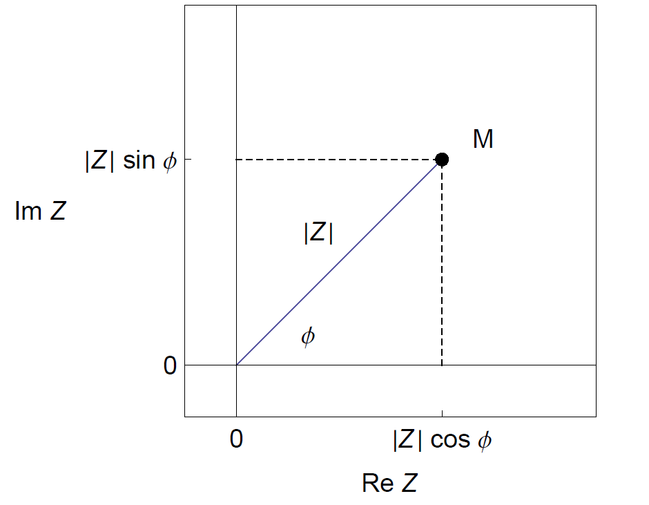
A complex number can be viewed as a point in a two-dimensional Cartesian1 coordinate system called the complex plane or Argand diagram [1], where the real part of Z is plotted as abscissa (Re Z = |Z| cos ϕ), and its imaginary part as ordinate (Im Z = |Z| sin ϕ). Z is the affix of M, M is the image of Z (Fig. 1).
Notations
Many notations of complex number can be found in literature, just some of these are noted below.
- Re Z, Im Z
- ℜZ, ℑZ
- Z′, Z′′
- ZRe, ZIm
- Zr, Zj
- |Z| cos(ϕ), |Z| sin(ϕ)
Complex Conjugate
a. Definition
The complex conjugate Z* of a complex number Z is defined by
$$Z=a+ib \Rightarrow Z^*=a-ib$$
b. Cartesian form of a complex number
Using the conjugate complex enables us to express complex numbers in the Cartesian (or rectangular or algebraic) form a + i b. For example, the Cartesian form of the inverse of a complex number is written:
$$\frac{1}{z}=\frac{1}{a+ib}=\frac{a-ib}{(a-ib)(a+ib)} = \frac{a-ib}{a^2+b^2}=\frac{a}{a^2+b^2}-i\frac{b}{a^2+b^2 } \tag{2}$$
Let us now consider the impedance of the electrical RC parallel circuit. It is given by [2]:
$$Z(\omega)=\frac{R}{1+RCi\omega} \tag{3}$$
With $\omega = 2\pi f$. Using Eq. (2), the rectangular form of the impedance of an RC parallel circuit is given by:
$$\begin{array}{l}
\text{Re}Z(\omega)=\frac{R}{1+C^2 R^2 \omega^2} \\
\text{Im}Z(\omega)=-\frac{CR^2 \omega}{1+C^2 R^2 \omega^2} \end{array} \tag{4}$$
Plots of Complex Function
Re(Z); Im(Z); vs. f OR log(f)?
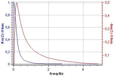
The real and imaginary parts of the impedance of an RC parallel circuit (Eq. (4)) depend on the frequency f. It is therefore possible to plot the change of the real and imaginary parts with the frequency f (Fig. 2)2. Please note that electrochemists usually plot −Im Z vs. Re Z, in such a way that that impedance diagrams are shown in the upper right-hand part of axes. From now on, in this note, we will use this type of representation.

Figure 2: Plots of Re Z vs: f and Im Z vs: f for the RC parallel circuit.
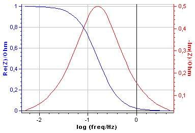
The frequency may vary over several decades. It is therefore better to plot the changes of Re Z and Im Z with the logarithm of the frequency, as shown in Fig. 3.

Figure 3: Plots of Re Z vs. log f and Im Z vs. log f for the RC parallel circuit.
Nyquist Plane
The diagrams shown in Fig. 3 can be plotted in a parametric plot with x = Re Z et y = Im Z. Such a graph is called Nyquist plot, Nyquist diagram or Nyquist graph. Each value of f determines a point (x = Re Z, y = −Im Z) that we can plot on a coordinate plane. As f varies, the point (x, y) varies and traces out a curve called a para-metric curve. A Nyquist plot is simply a para-metric plot of a frequency response.
a. Why use orthonormal axes?
Figure 4 shows the Nyquist diagram of the Randles circuit impedance [2, 3] plotted in cartesian orthonormal axes, i.e. axes with the same unit of length. It is made up of low frequencies of a semi-line forming a −π/4 or −45° angle (be careful, −π/4, due to the minus sign in the y coordinate, and not π/4 as the representation of electrochemists suggests) with the real axis and at high frequencies of an arc looking like a semi-circle.

Figure 4: Orthonormal Nyquist diagram for the Randles circuit.
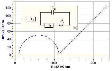

Figure 5: Non orthonormal Nyquist diagram for the Randles circuit.
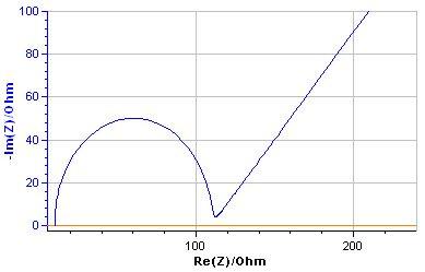
Figure 5 shows the impedance diagram of the Randles circuit for the values of parameters in Fig. 4, now using non-orthonormal axes. The semi-line at low frequencies does not form a −π/4 angle with the real axis and the high frequency arc is not a semi-circle any-more. It is easier to identify characteristic shapes using orthonormal axes. If a non-orthonormal representation is used then it must be explicitly justified as shown in [4, 5].
b. Why is the Nyquist diagram of the impedance of an RC parallel circuit a semi-circle?
The expression of the admittance, Y (ω) = 1/Z(ω), for an RC parallel circuit can be simply written:
$$Z(\omega)=\frac{R}{1+RCi\omega}\Rightarrow Y(\omega)=\frac{1}{Z(\omega)} = \frac{1}{R+Ci\omega}$$
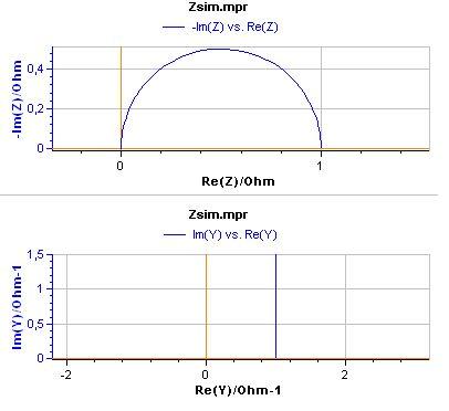
The Nyquist diagram of the admittance of the RC parallel circuit is made up of a semi-line (Fig. 6). The inverse of a semi-line is a semi-circle, therefore the graph of the impedance is a semi-circle.

Figure 6: Impedance and admittance diagrams of an RC parallel circuit.
c. Why specify frequencies on a Nyquist diagram?
The Nyquist diagram of Fig. 6 allows the determination of the value of the resistance R in the RC parallel circuit (R = 1 Ω). The value of the capacitance C cannot be determined, since no information about the frequency is given. What is needed is the value of the frequency of the point in the graph with the minimal imaginary part3 i.e. at the apex of the diagram. At this frequency fc :
$$C=\frac{1}{2\pi f_\text c R} \tag{5}$$
For $f_\text c$ = 1560 Hz, $C ~ 10^{-4}$ F.
Bode Plane
a. Modulus and phase plots
The modulus (also named module or magnitude) of an RC parallel circuit impedance is given by:
$$|Z|=\sqrt{(\text{Re}Z(\omega))^2+(\text{Im}Z (\omega))^2 )} = \frac{\sqrt{(R^2}}{\sqrt{1+C^2 R^2 \omega^2}}=\frac{R}{\sqrt{1+C^2 R^2 \omega^2}} \tag{6}$$
With (Fig. 7)
$$\lim_{\omega→0} |Z|=R,\omega\rightarrow \infty \Rightarrow |Z| \approx \frac{1}{C\omega} \tag{7}$$
The phase of an RC parallel circuit impedance is given by:
$$\phi_\text{Z}=\text{arctan} \left( \frac{\text{Im}Z (ω)}{\text{Re}Z (ω) } \right)=\text{arctan}(-CR\omega) \tag{8}$$
$$\lim_{\omega \rightarrow 0} \phi_\text{Z}=0,\lim_{\omega \rightarrow \infty} \phi_\text{Z}=-\frac{\pi}{2} \tag{9}$$

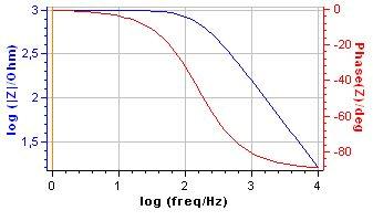
Figure 7: Bode magnitude and phase plots for an RC parallel circuit. R = 103 Ω, C = 10 6 F.
b. Why plot the impedance modulus and phase?
Measuring the impedance modulus change with the frequency is not sufficient to characterize an electrical circuit4. Figs. 7 and 8 show the Nyquist and Bode plots of an RC parallel circuit with R > 0 and R < 0, respectively.

Figure 8: Bode magnitude and phase plots for an RC parallel circuit. R = 103 Ω, C = 106 F.
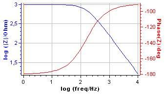
Such graphs commonly occur in corrosion protection, for example in the study of passivation phenomenon [7]. Modulus plots are identical but phase plots are different. The characterization of the electrical circuit is complete only if both the phase and the modulus are plotted. The reason lies in the term in Eq. (6). The value of the modulus is the same for R=103 Ω and R=-103 Ω. On the contrary the phase given by Eq. (8) depends on the sign of R.

Figure 9: Comparison of the impedance phase for R>0 (red) and R<0 (blue).
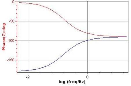
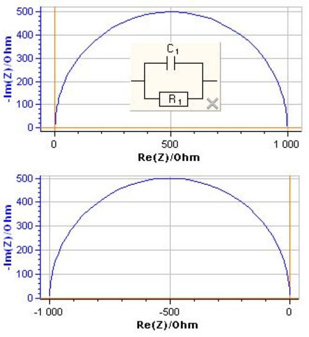
Figure 10 shows Nyquist diagrams for R > 0 and R < 0. The first diagram lies in the right hand side of the complex plane and the second in the left hand side.

Figure 10: Nyquist diagrams for a RC parallel circuit. C = 10 6 F, top: R = 103 Ω, bottom: R = 103 Ω.
Conclusion
Many representations are available to show impedance data due to them having complex values. Depending on the information of interest, the user can pick the right representation. The advantages and drawbacks of the main plots, Nyquist and Bode, are shown in Tab. I.
Table I: Advantages and drawbacks of Nyquist and Bode plots.
| Advantages | Drawbacks | |
|---|---|---|
| Bode | Explicit frequencies | Two plots |
| Nyquist | One plot | Implicit frequencies |
References
1) http://en.wikipedia.org/wiki/Complex number.
2) Handbook of EIS: Diffusion impedances
3) Interactive equivalent circuit library.
4) D. A. Harrington, J. Electroanal Chem., 355 (1993) 21.
5) V. M.-W. Huang, V. Vivier, M. E. Orazem, N. Pébère, and B. Tribollet, J. Electrochem. Soc. 154 (2007) C81.
6) Application note #15 “Two questions about Kramers-Kronig transformations
7) Application note #9 “Linear vs. non linear systems in impedance measurements”
Revised in 07/2018
[1] The invention of Cartesian coordinates is due to the French mathematician and philosopher René Descartes (1596-1650).
[2] All the figures were plotted using the simulation tool Z Sim from EC-Lab®.
[3] Not the maximum as the representation of the electrochemists suggests.
[4] In some cases, measuring the impedance modulus is enough as the plane can be deduced from Kramers-Kronig transformations, and vice versa [6].


