Obtain corrosion rate versus time automatically with the Corrosimetry technique!

Introduction

The determination of the corrosion rate provides information about the behavior of a system such as the impact of an environment over a material, or the protective ability of an electrodeposited coating for example. Polarization resistance techniques are widely used to determine the general corrosion rate of the studied electrochemical system. The Linear Polarization Resistance (LPR) technique is commonly used as a standard (ASTM G 59).

Following the corrosion rate with a potentiostat for a long period of time may help understand evolutions occurring at the electrolyte/material interface. Usually, this investigation may turn out to be laborious due to the repeated collection of data and the repeated analysis.

BioLogic’s single-channel or multichannel potentiostats / galvanostats do the measurements and the analysis automatically thanks to the EC-Lab^® “corrosimetry” technique which is described below.

Polarization resistance

The polarization of an electrochemical system consists of applying a voltage that is different from the equilibrium voltage of the cell. Depending on the polarization direction, it is referred to as anodic or cathodic polarization.

Using the Tafel theory, the polarization of the system (the overpotential) can be related to the current in the anodic area $\eta_\mathrm a=\log 10\; \beta_\mathrm a \log (i/i_0)$

and in the cathodic area $\eta_\mathrm c=-\log 10\; \beta_\mathrm c \log (i/i_0)$.

The Tafel parameters $\beta_\mathrm{c}$ can easily be determined with an experimental approach using the EC-Lab^® Tafel Plot technique and the EC-Lab^® Tafel Fit analysis tool. Other techniques are available in BioLogic’s potentiostat software to determine Tafel parameters such as the Variable Amplitude Sinusoidal micro Polarization (VASP) and the Constant Amplitude Sinusoidal micro Polarization (CASP). These techniques are described in Application Notes #36 and #37.

The polarization induces an increase of the rate of electrochemical reactions at the surface of the electrode and of the current flow, either anodically or cathodically. Resulting from this polarization, a polarization resistance is observed, which is the inverse of the slope of the stationary $I vs. E$ curve

$$R_\mathrm p = \dfrac{1}{\mathrm dI/\mathrm dE}\tag{1}$$

The Stern-Geary relationship establishes a correlation between the corrosion current and the polarization resistance in the vicinity of $E_{\mathrm{corr}}$.

$$I_{\mathrm{corr}}=\frac{B}{R_{\mathrm{p},E_{\mathrm{corr}}}}\tag{2}$$

With $$B=\frac{\beta_{\mathrm{a}}\beta_{\mathrm{c}}}{2.3(\beta_{\mathrm{a}}+\beta_{\mathrm{c}})}\tag{3}$$

And $\beta_{\mathrm{a}}$ and $\beta_{\mathrm{c}}$, the Tafel slopes.

For more details, see BioLogic Application Note #10: “Corrosion current measurement for an iron electrode in an acid solution” and BioLogic learning center topic: “Corrosion basics: determination of the corrosion current and potential”

Corrosimetry ($\boldsymbol{R_\mathrm p}$ vs. time)

The corrosimetry technique is available in the corrosion techniques section of EC-Lab^®. It is based on the Linear Polarization Resistance (LPR) technique, which permits to determine the polarization resistance. The Tafel parameters, $\beta_{\mathrm{a}}$ and $\beta_{\mathrm{c}}$, must be determined beforehand thanks to Tafel, VASP or CASP techniques and fill in the corrosimetry “Parameter Settings” window (Figure 1 below).

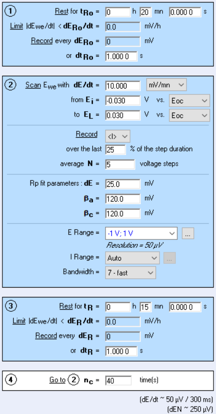
Figure 1: Corrosimetry “Parameter Settings” window

The corrosimetry technique allows the user to follow the evolution of the polarization resistance and the corrosion rate over a long period of time (up to several months) by automatically performing successive measurements of $R_\mathrm{p}$ (Fig. 2).

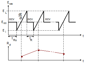
Figure 2: Diagram of the principle of the Corrosimetry technique

The user can also monitor the evolution of the corrosion rate of an electrochemical system. $R_\mathrm{p}$ and the corrosion rates are processed and displayed on-line, during the experiment. To do this, the equivalent weight, the density and the sample area must be correctly filled in the “Cell Characteristics” window (Figure 3 below) because these parameters are used in the calculation of the corrosion rate (see Equation 3).

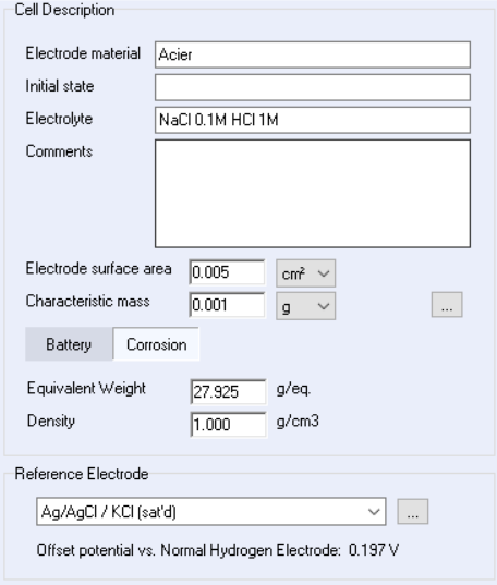
Figure 3: Corrosimetry “Cell Characteristics“ window

In the example presented in Figure 4, a corrosimetry experiment was performed on a piece of mild steel (undisclosed composition) immersed in a 1 M HCl solution with 0.1 M NaCl as a supporting electrolyte. The experimental set-up involves a BioLogic SP-150 single-channel potentiostat/galvanostat and a coating cell (EL-COAT). The $R_\mathrm{p}$ value (blue curve) increased with time (Figure 4, blue curve). As expected, the corrosion rate decreased with time (Figure 4, red curve). For the definition of the corrosion rate see the BioLogic learning center topic: “Corrosion basics: determination of the corrosion current and potential

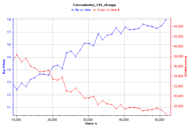
Figure 4: Corrosimetry curve $\pmb{R}_\mathbf{p}$ and $\pmb{CR}$ vs. time

The calculations of the polarization resistance and the corrosion rate is automatically performed by the EC-Lab^® software from the corrosion data, collected during the experiment, and the Tafel parameters. There is no need to post-process the data.