

Staircase Potentio Electrochemical Impedance Spectroscopy (SPEIS) and automatic successive ZFit analysis Battery – Application Note 18
Latest updated: May 2, 2023Abstract
In this application note, automation of successive ZFit analyses within EC-Lab® are demonstrated on staircase potentio EIS (SPEIS) experiments, as well as repetitive potentio EIS (PEIS) acquired at different times on non-stationary electrochemical systems. In both types of EIS experiments, successive experiments are performed using a simplified protocol, creating the need for equivalent circuit analysis on each one. ZFit provides a selection for “all cycles” to be analyzed within a given experiment, and plots the successive values for each component in the selected model for an even deeper analysis. The same process can also be applied to Galvano EIS as well as SGEIS.
Introduction
It is sometimes useful to automate measurements. With EC-Lab® and EC-Lab® Express, it is possible to automatically perform successive impedance measurements during a potential sweep with the SPEIS (Staircase Potentio Electrochemical Impedance Spectroscopy) technique. This technique allows the user to carry out different potential steps in the same experiment and, for each one, perform an electrochemical impedance spectroscopy measurement. For each experiment, the user defines the conditions. The main application of this technique is to study electrochemical reaction kinetics along steady-state curves. Note that the same process can be used in galvanostatic mode with the SGEIS technique.
Experimental Part
In the first part of this application note, the measurements were carried out on circuit #2 of the BioLogic Test Box 3. This circuit is non-linear as explained in ref. [1]. Measurements were carried out with the SPEIS technique of the EC-Lab® software (Figure 1).
This protocol allows the user to define the initial and final potentials (first and fourth blocks) with a number of EIS measurements (N) between the two limits. The second block allows the user to define the waiting time before the EIS experiment. The third block is relative to the EIS experiment and the definition of the EIS settings.
EIS settings are as follows: frequency sweep from 100 kHz to 50 mHz with 6 points per decade and a peak to peak amplitude of 5 mV.
Pw and Na were set, respectively, to 1 and 2 to let the system come back to a steady-state transient period after each frequency measurement and to have an average recorded value.
Note that this experiment takes ca. 2 h.
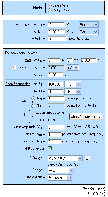
Figure 1: SPEIS “parameters Settings” window.
Determination Of The Diode Parameters Value
Cyclic voltammetry acquisition was performed between – 0.2 and 0.2 V vs. Ref on the circuit #2 of the Test Box 3, as shown in Figure 2 (it is possible to load the setting in the EC-Lab® software data as Cyclic Voltammetry_Test Box 3_Circuit 2.mps).

Figure 2: Steady-state curve I vs. Ewe recorded using Cyclic Voltammetry technique.
This circuit, made mainly of two semi-conductor diodes [1], is a model for exponential non-linearity [2] and mimics the Butler-Volmer relationship for an electron transfer reaction without limitation by the mass transfer of the electroactive species. The current vs. potential steady-state characteristic of circuit #2 is given approximately by the following relationship:
$$I_D = I_s(\mathrm{exp}(b_1(E-E_{I=0})) – \mathrm{exp}(-b_2(E-E_{I=0}))) \tag{1}$$
or in the form of the Stern relationship [3]:
$$I_D = I_s(10^{(E-E_{I=0})/\beta_a}-10^{-(E-E_{I=0})/\beta_c}) \tag{2}$$
Is, βa, βc, and EI=0 can be determined using the Tafel Fit analysis of EC-Lab® software (Figure 3).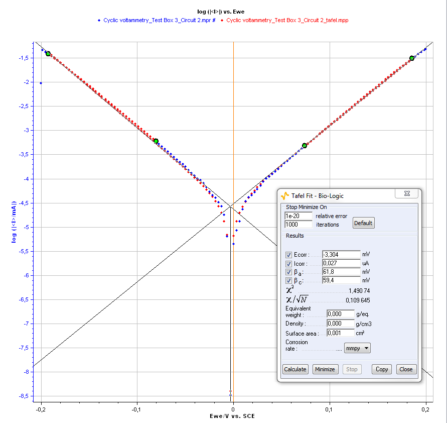
Figure 3: Tafel Fit Analysis.
The following values are obtained: EI=0 = – 0.003 V, IS = 2.7 x 10⁻⁸ A, βa = 0.062 V and βc = 0.059 V for the measurement on the circuit #2 of the Test Box 3.
Speis Measurement<
EIS experiments were carried out between – 0.1 and 0.1 V at each 10 mV potential step. Twenty-one impedance diagrams were measured in this potential range and shown in Figure 4 (it is possible to load the settings and the data files in the EC-Lab® software data as SPEIS_Test Box 3_Circuit 2.mps and SPEIS_Test Box 3_Circuit 2.mpr, respectively).
As expected, due to the shape of the current potential curve obtained with circuit #2 of the Test Box 3, impedance measurements are close on the anodic and the cathodic part, therefore impedance diagrams are grouped two by two.
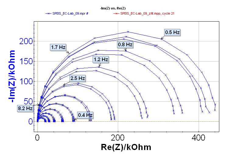
Figure 4: Nyquist impedance diagrams along the steady-state If vs. E curve.
Automatic Successive Fits
The ZFit analysis method allows the user to analyze impedance curves [3]. This tool can fit only one EIS curve of the series (Figure 5) or all the curves successively in an automatic fashion. The settings parameters are shown in Figure 6.
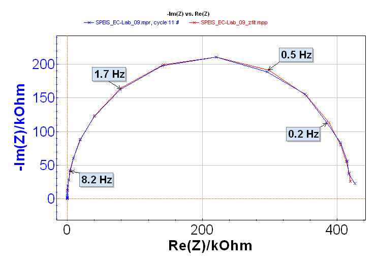
Figure 5: ZFit on the 11th Nyquist impedance diagram.
The equivalent electrical circuit selected in the ZFit window is given in Figure 7. It is composed of a resistance R1 in series with a capacitor C2 and a resistance R2 in parallel. Note that the value of R1 is constant along the potential range and is around 100 ? However, it is not the same for the other elements of this circuit due to its non-linearity. Indeed, the impedance of this non-linear circuit depends on the value of the working electrode potential Ewe, as showed in Figure 4.
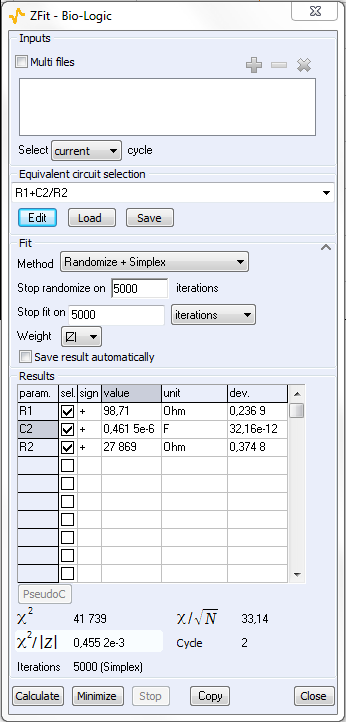
Figure 6: ZFit analysis window.
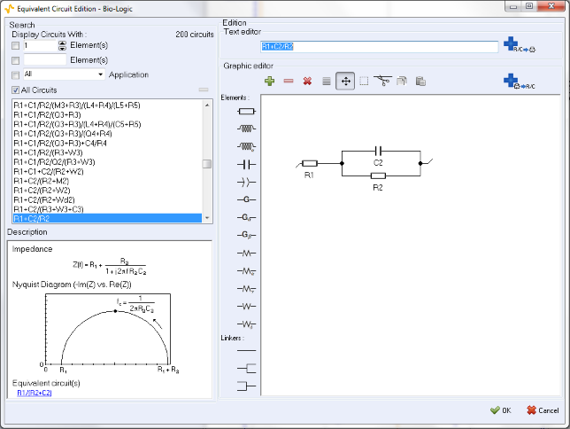
Figure 7: Electrical circuit selection in the ZFit analysis tool.
The ZFit tool allows the user to analyze each impedance diagram and plot the successive values of R2 and C2 values as a function of the working electrode potential. This result is given in Figure 8. R1 is not shown in this figure because as expected, the R1 value is constant along the potential range and close to 100 ? The value of C2 (ca. 0.46 x 10⁻⁶ F) is also constant along the potential range. It is shown with the R2 value change in Figure 8.
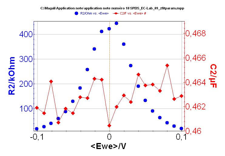
Figure 8: Changes of the R2 and C2 value vs. Ewe.
Determination Of The Circuit Parameter’s Value
Let us consider the change of R2 obtained using ZFit and the 21 Nyquist diagrams shown in Figure 8. For a low frequency input signal, the dynamic characteristic of the circuit#2 of the Test Box#3 is of the same form as the steady-state equation (1):
$$I_D(t) = I_s(10^{(E(t)-E_{I=0})/\beta_a}-10^{-(E(t)-E_{I=0})/\beta_c}) \tag{3}$$
Thus, the theoretical relationship for the charge transfer resistance for the circuit is given by:
$$R_{\mathrm t} = \left(\frac{\partial I_D}{\partial E}\right)^{-1} = \frac{1}{I_s \mathrm{ln}(10)\left(\frac{10^{(E-E_{I=0})/\beta_a}}{\beta_a}+\frac{10^{(E-E_{I=0})/\beta_a}}{\beta_c}\right)} \tag{4}$$
Considering the electrical circuit given in Figure 7 and the negligibility of R1 compared with R2, the previous relationship (4) can be written as:
$$R_\mathrm{p} = \left(\frac{\mathrm{d} I_\mathrm{D}}{\mathrm{d} E}\right)^{-1} = R_{\mathrm{t}} \tag{5}$$
with $R_s = R_\mathrm{p}$.
It is thus possible to determine the Is, βa, βc, and EI=0, values using a fitting procedure such as NonlinearRegress in Mathematica software. The results are shown in Figure 9.
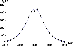
Figure 9: Comparison of experimental data taken from Figure 8 (dots) and theoretical curve (solid line) calculated for Is = 2.97 x 10⁻⁸ A, βa = 0.059 V, βc = 0.064 V and EI=0 = 0.0032 V.
These results show the good agreement between the dynamic state (experimental data) and the steady state (simulated data).
It means that steady state relationships can be used to describe the dynamic behavior of the system.
Automatic Zfit Analysis Of Non-Stationary Electrochemical System
Sometimes, electrochemical systems such as corroding electrodes, batteries, or electrochemical cells operating in finite dimensions media, are non-stationary, i.e. they change with time. Automatic ZFit can be used to study this change of the electrochemical system with time.
An example of the change with time of a system is given in Figure 10. These 16 successive Nyquist diagrams are recorded on the diffusion plateau during the oxidation of NaBH4 [5-7]:
$$\textrm{BH}_4^- + 8\textrm{OH}^- \rightarrow \textrm{BO}^-_2 + 6\textrm{H}_2\textrm{O} + 8\textrm{e}^-$$
All the Nyquist diagrams present the same shape and are made of two capacitive loops with decreasing modulus with time. EIS measurements were carried out using the PEIS protocol, the measurement period was repeated 15 times. Setting parameters are shown in Figure 11.
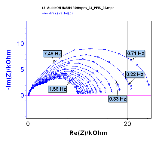
Figure 10: Nyquist impedance diagrams plotted on the diffusion plateau for the NaBH4 oxidation on an Au rotating disk electrode. Courtesy of G. Parrour and M. Chatenet/LEPMI.
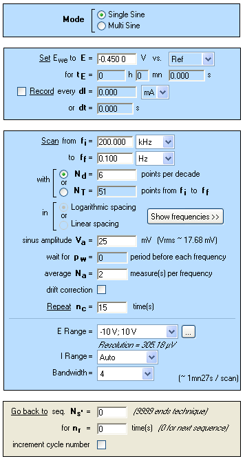
Figure 11: PEIS “parameters Settings” window.
Analysis of the Nyquist diagram changing with time can be made using the ZFit tool of EC-Lab® (or EC-Lab® Express) software. The Randles circuit R1+C2/(R2+Wd2) was selected (Figure 12) taking into account the shape of the Nyquist impedance diagrams (Figure 10). An example of the fit is given in Figure 13 for the 16th impedance diagram.
It is then possible, using ZFit, to automatically plot the change of R1, C2, R2, Rd2 or td2 as a function of the number of Nyquist diagrams. As an example, the changes of R2, Rd2 and C2 are shown in Figure 14.
As a consequence, automatic ZFit analysis of successive impedance diagrams can be used for monitoring non-stationary electro-chemical systems such as corroding electrodes or batteries.
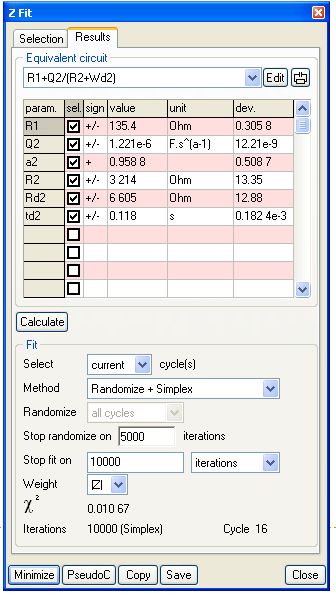
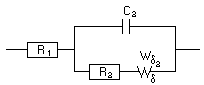
Figure 12: Equivalent circuit and ZFit analysis window.
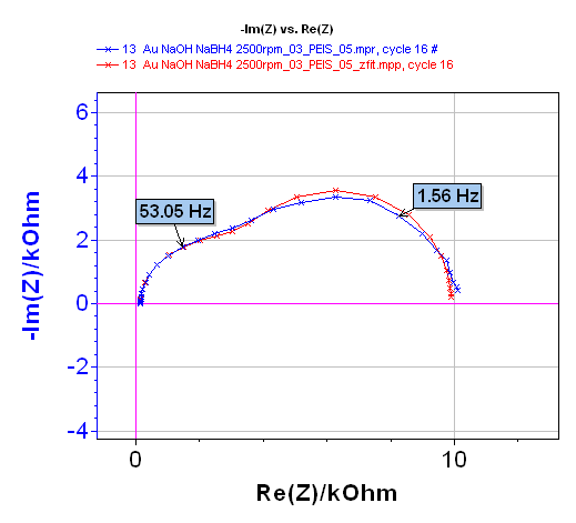
Figure 13: 16th Nyquist diagram (blue) and result of the fit (red).
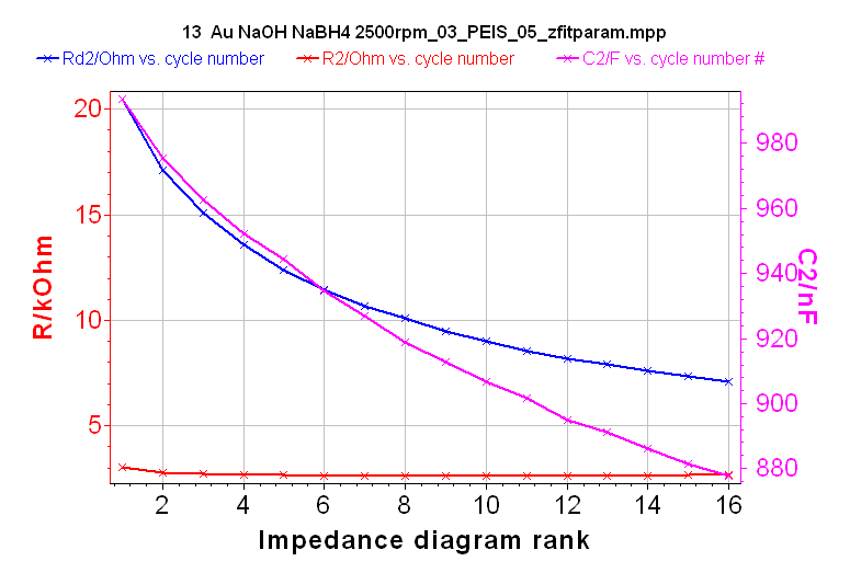
Figure 14: Change with time of R2, Rd2, and C2
Conclusion
The SPEIS method allows the user to automate EIS measurements along a steady-state or a non-stationary curve. Moreover EC-Lab® (or EC-Lab® Express) software is a well-adapted tool to simultaneously analyze successive impedance diagrams. EC-Lab® software (or EC-Lab® Express) allows the user to simplify experimental protocols and data treatments.
Data files can be found in :
C:\Users\xxx\Documents\EC-Lab\Data\Samples\EIS\AN18_
References
- Application Note #9 “Linear vs. non-linear systems in impedance measurements”
- J.P. Diard, B. Le Gorrec, C. Montella, J. Electroanal. Chem., 432 (1997) 27-39.
- Application Note #10 “Corrosion current measurement for an iron electrode in an acid solution”
- Application Note #14 “ZFit and equivalent electrical circuits”
- M. Chatenet, F. Micoud, I. Roche, E. Chainet, Electrochim. Acta, 51 (2006) 5459.
- M. B. Molina-Concha, M. Chatenet, J.-P. Diard, in: C. Gabrielli (Ed.) Proceedings of the 20th Forum sur les Impédances électrochimiques, Paris (2007).
- G. Parrour, Etude du mécanisme d’électrooxydation du borohydrure de sodium, Rapport de Master, Institut Polytechnique de Grenoble, 2008.
Revised in 04/2023


