

EIS Mathematics #2 – (The simplicity of Laplace transform) Battery – Application Note 50-2
Latest updated: July 8, 2025Abstract
The Laplace transform and its inverse are widely used in electrochemistry. This note illustrates some of its applications in DC or EIS measurement.
Introduction
Several electrochemical techniques use results obtained using the Laplace transform. Examples can be found in Application notes #21, #28, #38 and #41b [1-4].
Definitions
The Laplace1 transform of a function f(t) is defined by the integral
$$F(s)= \text L \{f(t)\} = \int^{\infty}_0 f(t)\text{exp}(-st)\text d t\tag{1}$$
Where s is the Laplace complex variable [5]. For example the Laplace transform of the sine function sin(t) is given by
$$\int^{\infty}_0 \text{sin}(t)\text{exp}(-st)\text d t\tag{2}$$
On the other hand, the time function is given by a more complicated expression from the Laplace transform in the s-domain by
$$f(t)= \text L^{-1} \{f(s)\} = \frac{1}{2 \pi i} \lim\limits_{T \to \infty} \int^{\gamma + iT}_{\gamma – iT}\text{exp}(st)F(s)\text{d}s\tag{3}$$
Table Of Laplace Transforms
Calculation of the integral of a function of a real variable is sometimes easy, e.g. it is well known that $\int xdx = x^2/2$. Calculation of the integral of a function of a complex variable is much more difficult. Fortunately it is very rare to have to use Eqs. (1) or (3). Laplace transforms and inverse Laplace transforms usually used in electrochemistry have already been calculated. The result is obtained by consulting a table of Laplace transform [5] (Tabs. I and II), or better using a software such as Wolfram Alpha [6].
Transfer Function of a Linear and Time Invariant (LTI) System
Definition
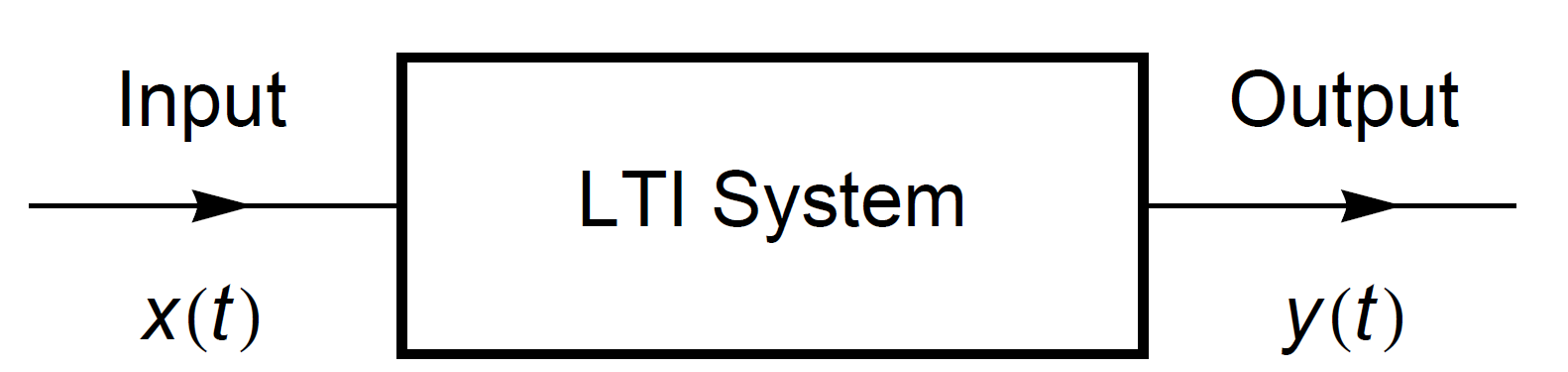
Laplace transform is the tool of choice for the study of linear and time invariant systems (Fig. 1) characterized by their transfer function H(s) defined by [7, 8]
$$H(s)= \frac{Y(s)}{X(s)} = \frac{\text{L}\{y(t)\}}{\text{L}\{x(t)\}}\tag{4}$$

Figure 1: Sketch of a scalar dynamic system.
For example, the impedance of a dipole is the transfer function for a current input
$$Z(s)= \frac{\text{L}\{\Delta E(t)\}}{\text{L}\{\Delta I(t)\}}= \frac{\Delta E(s)}{\Delta I(s)} \tag{5}$$
With $\Delta E(t)= E(t)-E_{t=0}$ and $\Delta I(t)= I(t)-I_{t=0}$.
Response of a LTI System
Introduction
Knowing the transfer function of a system allows us to calculate its response to an input. For example, if Z(s) is known, it is possible to determine the response of the dipole in the Laplace domain
$$\Delta E(s)= \Delta I(s)Z(s)\tag{6}$$
Then in the time domain using inverse Laplace transform
$$\Delta E(t)= \text L^{-1}\{\Delta E(s)\}\tag{7}$$
Response of a Parallel RC Circuit to a Current Heaviside Step Function
a. Impedance of a parallel RC circuit
The impedance of a parallel RC circuit is directly written from the admittance Y(s) = 1/Z(s) [9]:
$$Y(s)= \frac{1}{R}+sC \implies Z(s)= \frac{R}{1+RCs} \tag{8}$$
b. Response to a Heaviside step function
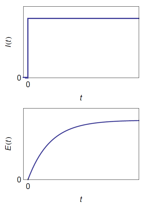
The Heaviside step function is equal to 0 for t<0 and 1 for t>0 (Fig. 2). The Laplace transform of the Heaviside step function is given by (Tab. I, Eqs. (1) and (2)).

Figure 2: Potential response of the parallel RC circuit to a Heaviside step current using Eq. (11).
$$\Delta I(s)= \text L \{\delta I(t)\} = \frac{\delta I}{s} \tag{9}$$
The Laplace transform of the output is written
$$\Delta E(s)= \frac{\delta I}{s} \frac{R}{1+RCs} \tag{10}$$
And the time domain response is given by (Tab. II, Eqs. (1) and (2)):
$$\Delta E(s)= \text L^{-1} \{\Delta E(s)\} = \text L^{-1} \left\{\frac{\delta I}{s}\frac{R}{1+RCs}\right\}= \delta IR \left( 1- \text{exp}\left(\frac{-t}{CR}\right) \right) \tag{11}$$
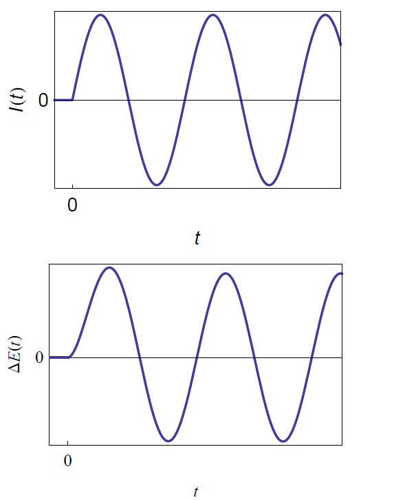
c. Response to a sinusoidal input
The Laplace transform of a sinusoidal signal is given by (Tab. I, Eqs (1) and (4))
$$I(t) = \delta I \text{sin}(\omega t) \implies I(s) = \text L\{\delta I(t)\}= \frac{\delta I \omega}{s^2 + \omega^2} \tag{12}$$
Therefore the output potential in the Laplace domain is
$$\Delta E(s) = \frac{\delta I \omega}{s^2 + \omega^2}\frac{R}{1+RCs}$$
And the time domain response is given by (Tab. II, Eqs. (1) and (4))
$$\Delta E(t) = \text L^{-1}\{\Delta E(s)\}= \text L^{-1}\left\{\frac{\delta I \omega}{s^2 + \omega^2}\frac{R}{1+\tau s}\right\} = \frac{\delta IR \left(\tau\omega\text{exp}\left(\frac{-t}{\tau}\right)\right)-\tau\omega\text{cos}(\omega t) + \text{sin}(\omega t)}{1+\tau^2\omega^2}\tag{13}$$
With τ = RC. The establishment of the sinusoidal steady-state of potential is shown in Fig. 3.

Figure 3: Potential response of the parallel RC circuit to a sinusoidal current using Eq. (13).
Ramp Response of a Series RC Circuit
a. Impedance of a series RC circuit
The impedance of a series RC circuit is given by
$$Z(s)= R+\frac{1}{C_s}\tag{14}$$
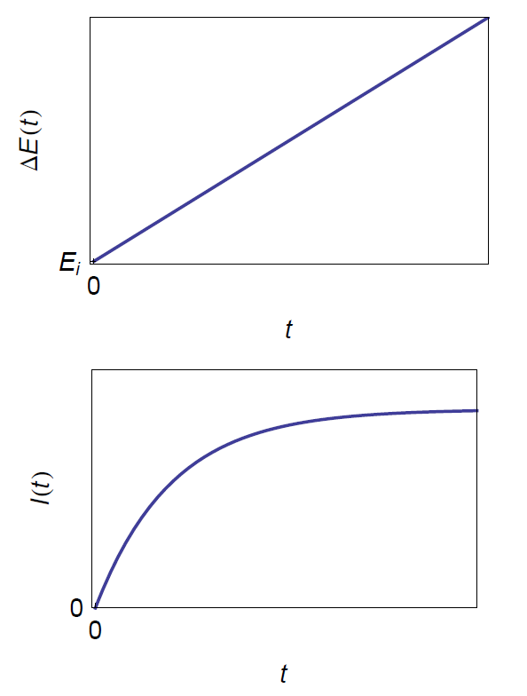
b. Response to a potential ramp
The signal used in linear sweep voltammetry is a potential ramp defined as:
$$E(t)=E_i+\upsilon t \implies \Delta E(t) -E_i= \upsilon t \tag{15}$$
The Laplace transform of a ramp is given by (Tab I., Eqs. (1) and (3))
$$\Delta E(s) =\text L \{\Delta E(t)\} =\text L \{\upsilon t\} = \frac{\upsilon}{s^2}\tag{16}$$
With
$$Z(s)= \frac{\Delta E(s)}{\Delta I(s)} \implies \Delta I(s) =\frac{\Delta E(s)}{Z(s)}$$
It is obtained
$$\Delta I(s) =\text L^{-1}\{\delta I(s)\} =\text L^{-1} \left\{\frac{C\upsilon}{s(1+CRs)}\right\}$$
And using Eqs. (1) and (2) (Tab. II),
$$\Delta I(t)= I(t)=C\upsilon\left( 1- \text{exp}\left(\frac{-t}{CR}\right) \right) \tag{17}$$

Figure 4. Current response of the series RC circuit to a ramp of potential calculated using Eq. (17).
Laplace and Inverse Laplace Transforms Tables
Laplace Transforms
Laplace transforms used in this note are shown in Tab. I.
Table I: Table of Laplace transforms.
| $$f(t)$$ | $$F(s)$$ | |
|---|---|---|
| (1) | $af(t)$ | $aF(t)$ |
| (2) | $1$ | $\frac{1}{s}$ |
| (3) | $t$ | $\frac{1}{s^2}$ |
| (4) | $\text{sin}(\omega t)$ | $\frac{\omega}{s^2 + \omega^2}$ |
Inverse Laplace Transforms
Inverse Laplace transforms used in this note are shown in Tab. II.
Table II: Table of inverse Laplace transforms.
| $$f(t)$$ | $$F(s)$$ | |
|---|---|---|
| (1) | $af(t)$ | $aF(t)$ |
| (2) | $\frac{1}{s(1+as)}$ | $1 -\text{exp}(-t/a)$ |
| (3) | $\frac{1}{s(1+as)}$ | $a(\text{exp}(-t/a)-1)+1$ |
| (4) | $\frac{1}{(1+as)(1+bs^s)}$ | $\frac{a \text{exp}(-t/a)-a \text{cos}(t/\sqrt{b})+\sqrt{b}\text{sin}(t/\sqrt{b})}{a^2 + b^2}$ |
References
1) Application note #21 “Measurement of the double layer capacitance”
2) Application note #28 “Ohmic drop. Part II: Introduction to Ohmic Drop measurement techniques.”
3) Application note #38 “Dynamic resistance determination. A relation between AC and DC measurement?”
4) Application note #41 II “CV Sim, Simulation of the simple redox reaction (E), Part II: The effect of the ohmic drop and the double layer capacitance.”
5) http://en.wikipedia.org/wiki/Laplace_transform.
6) Wolfram Alpha: Computational Knowledge Engine. http://www.wolframalpha.com.
7) http://en.wikipedia.org/wiki/Transfer function.
8) Handbook of EIS – Transfer functions.
9) Handbook of EIS – Circuits made of resistors and capacitors.
Revised in 07/2018
1Pierre-Simon Laplace was a French mathematician of the eighteenth century (1749-1827).


