
Stopped-Flow & Deadtime: Everything you need to know
Latest updated: June 2, 2023What is dead time?
The dead time of a stopped-flow instrument is the time it takes for the solution to pass from the center of the mixer, where the reaction starts, to the observation point. This is the part of the reaction you do not see in your stopped-flow recordings. So the lower the dead time, the more you see and the more information you can generate.
You will find below an example of a trace (figure 1) you can obtain with a 8 ms dead time, the data looks good and it could be fitted perfectly using a single exponential.
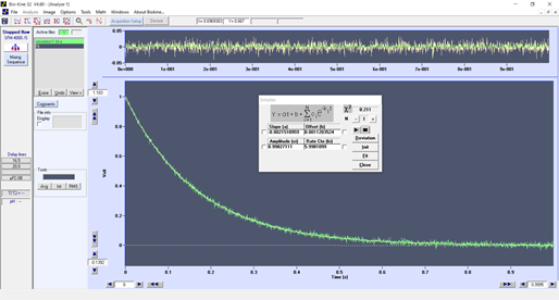
Figure 1 : stopped-flow experiment with a 8 ms dead time
However, if we perform the same reaction with a 1 ms dead time (figure2), the trace looks completely different and shows an initial decay during the first 8 ms. The model is clearly not a single exponential anymore. Without a short dead time you would have missed this initial data and it could have led you to misinterpret your reaction mechanism.
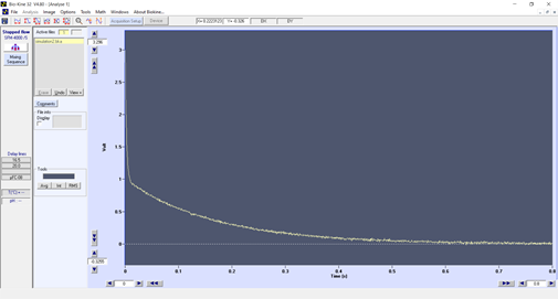
Figure 2 : same stopped-flow experiment with a 1 ms dead time
The zero point on the time axis does not correspond to the start of the reaction, it corresponds to the initial age of the solution at the observation point: in other words, the dead time !
How do you measure dead time?
By definition, dead time is considered to be the cell volume (from the mixing point to the observation point) divided by the solution flow-rate. The cell volume is known and given in the users manual and the total flow rate is set by the user, thanks to the stepping motors. The dead time can therefore be estimated by the software for each experiment. It is an estimated value as there could always be a small deviation in the real cell volume because of O-ring compression or some hydrodynamic phenomena.
This deviation on dead time is in the range of 0.1 to 0.2 ms. For most reactions the user can trust the estimated value, as not much would happen during this time. But for very fast reactions (where some signal changes can be observed during this time) the experimental dead time needs to be precisely determined.
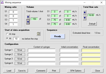
Figure 3 : example of stopped-flow sequence
This could be easily performed by choosing a fast reaction that follows an exponential decay. First you mix the sample with the buffer to obtain the maximum signal amplitude expected. Then you run your kinetics and fit your trace with a single exponential. You obtain a rate constant and a signal amplitude. If the dead time was 0, this amplitude would match the amplitude of the dilution. The missing part of the signal is the reaction that occurs during the dead time. Therefore, by extrapolating the exponential it is possible to determine the time shift on the time axis: this is the dead time.
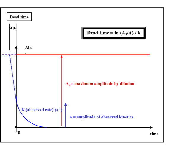
Figure 4: experimental method to determine the dead time
What is the minimum dead time?
The dead time of the stopped-flow is directly linked to the size of the cuvette you are using. In most configurations the dead time is between 0.5ms and 1 ms. But using the microcuvette accessory you can reach 200µs dead time. This performance is not only due to the cuvette’s small volume but to the mixing and pushing technology, as the mixing process must be completed much faster than the dead time. Some detection techniques like neutron scattering or FT-IR require larger cells to have sufficient sensitivity so that dead time can be a couple of milliseconds.
Other considerations
Dead time is important, but if you want to exploit its full benefit, you need to ensure that the time resolution of the spectrometer you use is faster. For example, if your stopped-flow has a 0.2 ms dead time but you collect data every 10ms, then the effective dead time will be 10 ms! This is why most bench spectrometers or fluorimeters cannot be used efficiently for stopped-flow studies. BioLogic offers a range of spectrometers specially developed for rapid kinetics with acquisition speeds optimized for stopped-flow. So, by combining 200µs dead time and 10µs data sampling you can easily observed reaction finished in a couple of milliseconds.
The video below may also be of interest with regards to this article.
Broaden your scope! The following articles may be of interest...
Related products